|
Multiple regression related the dependent variable Y to a number of independent variables, for example Y = A1 * X1 + A2 * X2 ... +B. Non linear or polynomial regression provides relationships that involve powers, roots, or other non-linear functions, such as logarithms or exponentials. Excel and Lotus 1-2-3 offer some simple linear and non-linear regression models, but more sophisticated software is required for multiple regression. A good freeware package is Statcato (www.statcato.org). It is a java based program: right-click and "Save Target As" >> Stats / Regression Package, unzip the files to a folder, and click "Statcato.jar".
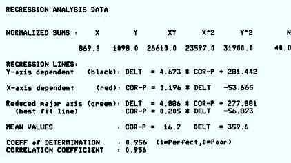
The "X-on-Y line reverses the roles of the two axes, minimizing the error in the horizontal direction (as the graph is drawn here).. The RMA line, the reduced major axis, assumes that neither axis depends on the other and is very nearly halfway between the first two lines. It minimizes the error at right angles to the line. The ER, or error ratio line, minimizes the error on both X and Y directions. There is not usually much difference between the RMA and ER lines. All four lines intersect at the centroid of the data.
The
Reduced Major Axis regression line is the regression line that
usually represents the most useful relationship between the X
and Y axes. It assumes that both axes are equally error prone.
An approximation to this line is halfway between the two independent
regression lines. Solve equation 6 for Y: Average
slope and intercept of equations 5 and 7: Coefficient
of Determination The coefficient of determination is a measure of "best fit" and is capable of being calculated as data is entered and processed (e.g.: as in a hand calculator). Other measures of fit require two passes through the data - the first to find the average X and average Y values, then a second pass to find the differences between each individual X and the average X, and the differences between the individual Y and the average Y values. An
alternate form of the above equation is: Both equations give the same answer. These data are used in the following statistical measures. Arithmetic
Mean Variance
Standard
Deviation Correlation
Coefficient T
Ratio Skew
Kurtosis
Geometric
Mean Harmonic
Mean Where:
The b's are termed the "regression coefficients". Instead of fitting a line to data, we are now fitting a plane (for 2 independent variables), a space (for 3 independent variables). The estimation can still be done according the principles of linear least squares. The algebraic formulae for the solution (i.e. finding all the b's) are UGLY. However, the matrix solution is elegant: The matrix model is:
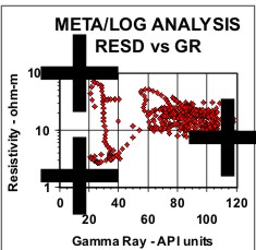
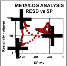
Statistical analysis of data, such as regression analysis or frequency distributions, can be described both graphically and mathematically. The math for very basic statistical analysis of petrophysical data is covered here. The majority of crossplots are X - Y coordinate graphs, often called scatter plots. They are useful for showing the relationship between two measurements, for example, resistivity versus gamma ray readings. By making the symbol that is plotted vary in colour with a third parameter, for example the PE curve, we have a 3-D crossplot. In this case it shows the variation of lithology with changes in resistivity and gamma ray value. Although not widely used, the shape of the characters used to plot each data point can be varied to represent a fourth variable, for example the frequency of occurrence of data at this location on the plot. These are 4-D plots, invented by the author in 1976. Groupings of data may represent important petrophysical parameters, such as shale properties, water or hydrocarbon zone location, or mineralogy. The use of a particular crossplot is dictated by common sense rules. Some crossplots, especially those related to mineralogy, benefit from a background template showing the location of the pure mineral values observed in the laboratory.
Regression analysis of log data, or core versus log data, is very commonly used to find relationships that predict or calibrate petrophysical results, as at the right. The equation of the best fit line can be used in user-defined equation sets in most computer or spreadsheet software.
The other common crossplot with core data are regressions of core porosity against sonic, density, neutron, or answer porosity, used to establish calibration equations.
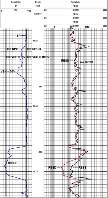
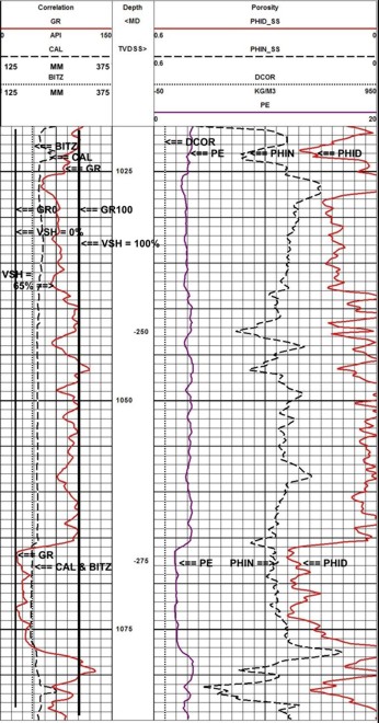
The raw logs show two zones of interest: a lower clean sand with hydrocarbon over water and a very poor quality upper shaly zone with a hydrocarbon indication. These zones can be spotted by laying the density log over the resistivity log and looking for the crossover of the curves. Because the sands are not pure quartz, a conventional shaly sand analysis technique is not appropriate because it would underestimate porosity, so a complex lithology model was used instead.
There is no density neutron crossover in the clean sand, so this zone is oil bearing. We cannot tell about the upper shaly sand because the shale effect masks any possible gas effect. After shale corrections, the density and neutron still do not cross over, so oil is most likely.
The water zone at the base of the clean sand provides water resistivity information for use throughout the rest of the zone. Core data was available to calibrate porosity and permeability results. The answer plot shows the results of the lithology, porosity, and hydrocarbon analysis.
The raw data plot shows two interesting features: the flat SP compared to GR in tight zones and the SP excess at 3400 feet, indicating better permeability than the rest of the shaly sand. The lithology track on the answer plot shows this interval to be more sandy and less limey than the rest of the shaly sand.
Raw logs for Shaly Sand Example
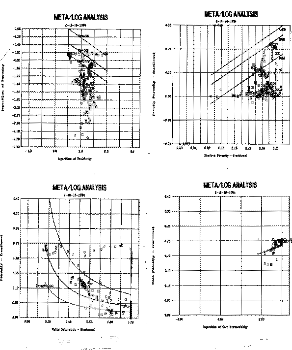
The following crossplots were made:
1.
Porosity vs Resistivity - shows
water saturation lines (shale data falls below 100% Sw line).
2.
Porosity vs Saturation - shows
constant water volume lines. Data streaming above and to the
right indicate transition and water zones. Shale data falls to
the bottom of the graph.
3.
Density vs Neutron - shows all data
below limestone line, indicating either no perfectly clean sand
or mixed lithology sand (GR suggests clean sand). Shale data
falls towards bottom and right. 4. Core porosity vs core permeability - shows a data cluster which cannot be used to derive a regression line mathematically. A line drawn thru the lower left corner will work fine.
Basic crossplots for Shaly Sand Example - Part 1
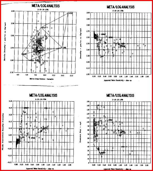
5. Matrix density vs matrix cross section - confirms that sand is not pure quartz, but the plot does not tell us which minerals to expect. Sample description suggests quartz, calcite, and glauconite (plots past anhydrite at top right).
7.
Apparent water resistivity vs
density porosity - similar to above but uses effective porosity.
Shale plots near origin, water zone at top left, oil at right.
8.
Apparent water resistivity vs gamma
ray - shows where to pick GR0 and GR100 (also can be picked from
raw logs). Best oil zone is off scale to the right.
Basic crossplots for Shaly Sand Example - Part 2
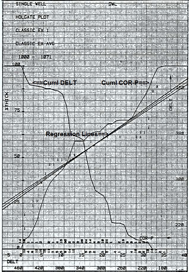
The data is sorted into ascending (or descending) values and placed into cells with discrete ranges:
The crossplot is created by plotting the lower row of numbers (the accumulated number of samples) on the Y axis versus the centroid of the range of data values represented on the X axis. Usually these points are connected by a series of straight lines. If the range of values in each cell is very small, a smooth cumulative curve can be created. This is normally done on a computer. If two such curves are made, one for a log value, and the other for a core property such as porosity, a calibration curve can be constructed. Assume our previous data reflected core porosity data and the sonic data had the following values:
The resulting calibration would relate the centroid of each range to its corresponding value in the other table. Thus:
A best fit regression analysis on this paired data would generate the equation of the line which calibrates sonic log readings to porosity. The relationship need not be linear. The data for the two sets of values must come from the same interval of rock, but the two sets do not need to be "on depth" with each other since no actual depth values are used. In fact, an upside-down core will still produce the same log calibration as a right-side-up core. Although
the Y-axis accumulations were a number of samples in this example,
the accumulation can be any one of: A
compact form of this plot comprises three separate plots on one
page, with axes appropriately labeled. The three plots are: The first two curves will create two "S" shaped curves facing in opposite directions and crossing at their median values. The third curve, when fitted with a regression line, will provide the calibration equation.
|
|
||||||||||||||||||||||||||||||||||||||||||||||||||||||||||||||||||||||
|
Page Views ---- Since 01 Jan 2015
Copyright 2023 by Accessible Petrophysics Ltd. CPH Logo, "CPH", "CPH Gold Member", "CPH Platinum Member", "Crain's Rules", "Meta/Log", "Computer-Ready-Math", "Petro/Fusion Scripts" are Trademarks of the Author |
|||||||||||||||||||||||||||||||||||||||||||||||||||||||||||||||||||||||

|
||
| Site Navigation | BASIC MATH REGRESSION STATISTICS and CROSSPLOTS | Quick Links |
 The graph at
left (courtesy Dick Woodhouse) shows four different lines. The "Y-on-X" line is the one
that will result from use of spreadsheet software. Y is the
dependent axis (predicted variable) and X is the independent axis
(the variable doing the predicting). The line minimized the errors
in the vertical direction (Y axis) using a least-squares solution.
The graph at
left (courtesy Dick Woodhouse) shows four different lines. The "Y-on-X" line is the one
that will result from use of spreadsheet software. Y is the
dependent axis (predicted variable) and X is the independent axis
(the variable doing the predicting). The line minimized the errors
in the vertical direction (Y axis) using a least-squares solution. Slope
of Best Fit Line
Slope
of Best Fit Line  Equation
of Best Fit Lines
Equation
of Best Fit Lines 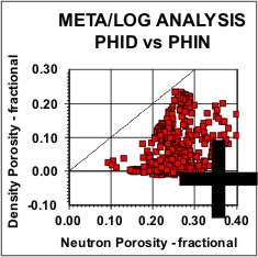
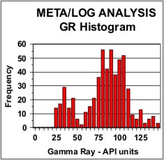 Histograms of the distribution of log
data are used for choosing petrophysical properties, as in the GR
example at left. They are also used to help in normalizing log data
between wells by suggesting the linear shift needed to match the
distribution from a model or key well.
Histograms of the distribution of log
data are used for choosing petrophysical properties, as in the GR
example at left. They are also used to help in normalizing log data
between wells by suggesting the linear shift needed to match the
distribution from a model or key well.