|
 DECLINE CURVE BASICS
Virtually all oil and gas wells produce at
a declining rate over time. The initial flow rate may be
held constant on purpose (restricted rate) or the decline
may begin immediately. The ultimate recovery from the well
(reserves) can be calculated by projecting the decline rate
forward in time to an economic limit. The projected
production can be summed to find the total production on
decline, and this can be added to the production during the
constant rate period to obtain the ultimate recovery.
This can be done on a per well basis
or for an entire reservoir. The result can be used as a control on
the volumetric reserves calculated from log analysis results and
geological contouring of field boundaries. It is often used to
estimate the recovery factor by comparing ultimate recovery with
original oil in place or gas in place calculations.
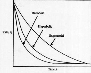 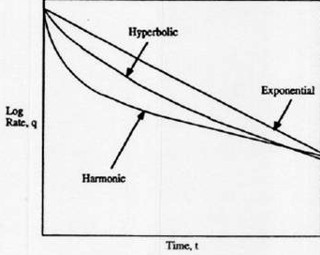
Production history plot: linear (cartesian coordinate (left),
semi-logarithmic plot (right). Most oil wells and some gas wells
produce with an exponential decline (straight line on logarithmic
plot). Some oil and gas wells decline at a faster rate, called
hyperbolic or double exponential decline. Still faster declines can
occur, especially in fractured reservoirs, called harmonic decline.
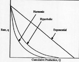
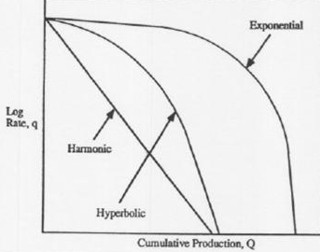
Cumulative production plot: linear (cartesian coordinate (left),
semi-logarithmic plot (right). Ultimate recovery is highest for
exponential decline
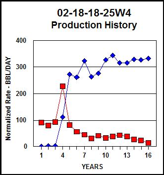
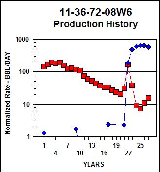
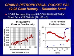
Production history graphs for two
real wells: linear scale (left), semi-log scale (right). Both show
restricted initial rate followed by exponential decline (red = oil, blue =
water production).
Determining decline rate and
Ultimate recovery```
Natural decline trend is dictated by the reservoir drive mechanism,
rock and fluid properties, well completion, and production
practices. Thus, a major advantage of this decline trend analysis is
inclusion of all production and operating conditions that would
influence the performance of the well. Conversely, predictions from
the decline history assumes that no significant changes in these
factors will take place.
The generalized decline curve is
described by::
1: D - Di * (Q / Qi)^N
Where:
D = instantaneous decline rate at time T
Di = initial decline rate
Q = instantaneous flow rate
Qi =initial flow rate at start of decline
N= 0 for exponential decline
= 1 for harmonic decline
= 2 for hyperbolic decline
Production as a function of time
on decline:
Exponential decline
2: Q = Qi * exp (-Di * T)
Harmonic decline
3: Q = Qi / (1 + Di * T)
Hyperbolic decline
4: Q = Qi / (1 + N * Di * T)
NOTE: Q, D, and T must be in compatible units (egL bbl/day, 1/day,
and days respectively, or month or year)
The cumulative production for each case is:
Exponential decline
 5: Np = (Qi - Q) / Di
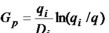 Harmonic decline
6: Np = (Qi / Di) * ln (Qi / Q)
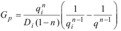
Hyperbolic decline
7: Np = (Qi^N) / (Di * (1 - N)) * ((1 / (Qi^(N -
1)) - (1 / (Q^(N - 1)))
Where:
Np = cumulative production to time T
Np is usually replaced by the symbol Gp when the reservoir is a gas
zone.
The time to abandonment for each case is:
Exponential decline
8: Ta = (1 / Di) * ln (Qi / Qa)
Harmonic decline
9: Ta = (1 / Di) * (Qi / Qa - 1)
Hyperbolic decline
10: Ta = (1 / (N * Di)) * ((Qi / Qa)^N - 1)
Where:
Ta = time to abandonment
Qa = production rate at abandonment
NOTE: To find ultimate recovery
(reserves), calculate abandonment time (Ta), then use Ta as the time
term in equations 5, 6, or7.
|