Analysis of water saturation became more reliable because of reduced borehole effect on the resistivity measurements, compared to conventional electrical resistivity logs. To some degree, bed boundary effects were more predictable and compensated for electronically. The induction log has evolved considerably over its fifty year life and is the most common log run today.
The electrical, SP, and gamma ray logs all measured the average value of rock properties over eighteen inches to five feet of rock thickness. Beds thinner than this could not be detected or evaluated. The microlog was introduced in 1948 and allowed resistivity in beds as thin as two or three inches to be measured at a correspondingly shallow depth of investigation into the rock. The log can be thought of as a miniature ES log supported on a rubber pad pressed tightly to the borehole wall. The curve shape approach to analysis was commonly used for microlog data, although laboratory derived charts allowed quantitative analysis of formation factor, and as a result, porosity. The curve shape analysis for micrologs provided rapid visual identification of zones which were invaded by drilling fluid, and were thus permeable to some small degree. The log is still used today for this purpose.
Microlog circa
1949. Shaded areas show good SP and "positive separation",
indicating permeable rock. Combined with high resistivity on the ES
log, this combination of logs could pinpoint oil or gas reservoirs.
The laterolog was also introduced in 1948 - 1949. It was a multi-electrode electrical log designed to minimize borehole effects in salty drilling mud. Again, improved resistivity values led to better water saturation and porosity determinations, still using the Archie method. The microlaterolog, to replace the microlog in salt mud, was first seen in 1952. Curve-shape analysis was not easy, but standard Archie methods worked well with this data. Other similar tools, such as the proximity log, and the micro-spherically focused log, are variations of the microlaterolog designed to improve shallow resistivity measurements in a variety of borehole conditions. Neutron logs first appeared in 1938, but were not common until l946, when better sources of neutron radiation became more readily available. Neutrons emitted by the source, are absorbed by hydrogen atoms, which are common in water and petroleum. Qualitative analysis of porosity (which contains water or oil) was possible by detecting the number of neutrons which were not absorbed but were scattered back to the detector. In some tools, the captured gamma rays created by the neutron bombardment were counted instead of the neutrons. This was the first independent source of porosity information that did not rely on Archie's formation factor concept and the resistivity log data. The tool had, and has, its faults, but modern neutron logs are useful quantitative analysis aids. Again, better detectors have increased the resolution and accuracy of the measurements. The modern version of the neutron log compensates for borehole size and a number of environment factors automatically. The two-receiver acoustic travel time (sonic) log showed up in 1957. Laboratory work had demonstrated that the travel time of sound in a rock, after adjustments for fluid and matrix rock travel time values, was capable of estimating porosity. Thus, another independent source of porosity data was born. M. J. Wyllie published an analysis method for apparent porosity from the sonic log using the time average equation in 1956. It is one of the most common analysis methods in use. The laboratory work and relationships between porosity and sound velocity (or travel time) was exhaustively studied between 1940 and 1965. Much of the work was aimed at solving problems in seismic survey analysis. Strangely enough, the Wyllie formula, for all its success over almost fifty years of use in log analysis, can be shown to be physically incorrect in the laboratory and in theory for many situations, especially those involving compressible fluids such as gas. The sonic-resistivity crossplot was invented shortly after the sonic log. It allowed visual as well as quantitative presentation of porosity and water saturation results on one piece of paper without the use of additional charts, nomographs, or slide rules (hand calculators had not yet been invented). It was tedious work, but thousands of crossplots were made during the sixties, and a few less progressive analysts still use them today.
Quick look methods to differentiate hydrocarbon zones from water zones also followed the introduction of the sonic log. One such technique, the "Rwa Method", is still very popular. The principle used was to quickly calculate, from the Archie water saturation equation and the sonic log porosity value, the apparent water resistivity which would make the zone 100% water saturated. If a particular value of water resistivity was considerably higher than the trend of many other values from above and below it in the borehole, then hydrocarbon could be suspected in the anomalous zone. No shale corrections were made, so shaly sands often showed poorly in this analysis. Another quick look method is called the overlay method. The simplest approach was to overlay the resistivity log and the sonic log in such a way as to have the two curves fall on top of each other in the obvious water zones. Zones in which the resistivity log fell to the right of the sonic log were either potential pay zones or tight (non porous). The overlay method was improved by generating compatible scale logs so that scaling differences did not cause false shows. The compatibility could be created by transforming the resistivity and sonic curves to apparent porosity or to apparent formation factor. This was done at the wellsite by appropriate function formers in the surface electronics, or back in the office by use of computer processing. The invention of the logarithmic presentation for resistivity data, when the dual induction log was introduced in 1962, made quick look overlay methods even more popular and practical at the well site. Many modern logs are designed to give good visual impressions of lithology, porosity, or hydrocarbon by means of compatible scale overlays. The density-neutron combination log is the most common example. The latest versions of computerized logging trucks even shade-in the separation between compatible scaled logs to emphasize the apparent prospective zones.
Since a crossplot is merely the solution to three simultaneous equations in three unknowns, the use of computers to solve these equations was a popular subject in the early sixties. Extensions of this concept to four, five or six simultaneous equations demanded a computer since graphical methods could not cope with the multi-dimensional aspect of the job. <==
Early Computed Log c. 1966 Linear programming (simultaneous equations with constraints) was tried. It was not very successful, because knowledge of rock properties, the so-called known data, was not really very well known. As well, tool response to rock mixtures was not well defined. The late fifties and early sixties also saw a great deal of work in atomic physics and both the pulsed neutron (or atomic activation) log and natural gamma ray spectroscopy log were described. However, suitable tools did not become available until 1968, and were not common until 1971. The pulsed neutron log provides another apparent porosity evaluation, as well as an independent assessment of water saturation. The logs are also called thermal decay time logs, chlorine logs, carbon/oxygen logs or spectral gamma ray logs (note the lack of the word "natural" in this case) depending on the details of the source-detector systems and the rock properties derived from the data. They are usually run in cased holes. The natural gamma ray spectrolog allows analysis of uranium, thorium and potassium content in a formation. This is used to help segregate shale from other naturally radioactive rocks, such as uranium bearing dolomites or potassium rich sandstones. In conjunction with other log data, it can help define the types of clay minerals present in the shales. The nuclear-magnetic resonance log was described in 1956. The theory suggested that effective porosity and permeability could be determined from the measurements. Good examples of this are still rare even after nearly fifty years of refinement- but Year 20XX versions of the tools will probably succeed. Unfortunately, the tool sees a very small fraction of the rock seen by other logs, so it may never be realistic to compare values from such dissimilar rock volumes. Other methods for interpreting permeability, based on empirical relationships between porosity and water saturation had been presented prior to l960 and are still used today. Some examples are the Timur, Wyllie-Rose, and Coates-Dumanoir methods.
Prediction of abnormal pressured zones, and potential drilling or blowout problems, were developed from the various porosity estimating logs, beginning in l956. This was based on depth-trend line analysis of the sonic log primarily, although most logs, including density, neutron, and resistivity logs can be used. The log types and analysis methods discussed so far are all used in open-hole conditions, that is, after the well is drilled but before it is cased with pipe and cement, and finally completed to flow oil or gas (or heaven forbid, water). All the radioactive logs (gamma ray, spectral gamma ray, neutron, pulsed neutron) except density logs can be run in cased holes, and interpreted with approximate corrections for casing size and thickness. Resistivity and older style sonic logs cannot be run in casing to obtain information about the rocks, although the sonic log is used to evaluate the cement behind the casing. Sonic wavetrain logs run through the casing are sometimes useful in evaluation of the rocks, but are most frequently used for cement evaluation. Recent versions of sonic logs use computer processing of the wavetrains to determine compressional, shear, and Stoneley wave travel times in both open and cased-hole situations. Resistivity logging through casing is also being developed. Other logs, such as temperature, flow-meter (spinner surveys), gradiomonometer (a fancy name for fluid density meter), and noise logs are used to assist in analysis of the location, amount, and type of fluid flow in producing or injecting wells. The tools and techniques have evolved gradually since l952, when the first serious effort was made to evaluate well performance with logging tools.
While the early years were clearly a period of invention of
hardware and techniques, the middle years could be termed the
period of understanding. Although significant new tools were
developed, such as the sonic and density logs, the
analysis process required more formidable effort.
Customers wanted more reliable answers along with the more
reliable logging tools. |
|
||
|
Page Views ---- Since 01 Jan 2015
Copyright 2023 by Accessible Petrophysics Ltd. CPH Logo, "CPH", "CPH Gold Member", "CPH Platinum Member", "Crain's Rules", "Meta/Log", "Computer-Ready-Math", "Petro/Fusion Scripts" are Trademarks of the Author |
|||

|
||
| Site Navigation | HISTORY WELL LOGGING 1946 - 1970 | Quick Links |
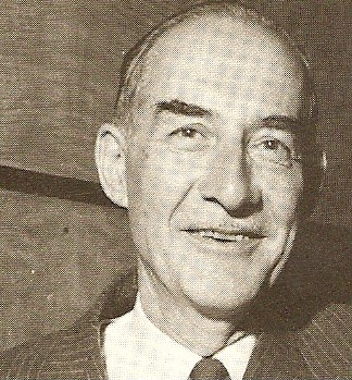 Henry
Doll of Schlumberger developed the induction log from research he
had performed to create the mine detector during World War Two. He
was also responsible for the invention of the microlog, laterolog,
and microlaterolog.
Henry
Doll of Schlumberger developed the induction log from research he
had performed to create the mine detector during World War Two. He
was also responsible for the invention of the microlog, laterolog,
and microlaterolog.
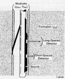
 The
density log was introduced in l959. It was another independent
source of porosity data. With three sources of apparent porosity,
(sonic, neutron and density), in addition to the resistivity methods,
it was now possible to account for more variables. This led to
crossplot or chartbook methods which compared the apparent porosity
values from two sources, to help identify lithology (shale content
or limestone - dolomite ratio, for example).
The
density log was introduced in l959. It was another independent
source of porosity data. With three sources of apparent porosity,
(sonic, neutron and density), in addition to the resistivity methods,
it was now possible to account for more variables. This led to
crossplot or chartbook methods which compared the apparent porosity
values from two sources, to help identify lithology (shale content
or limestone - dolomite ratio, for example). The
sonic-density crossplot was common in the early sixties, with
the density-neutron crossplot becoming more common in the late
sixties, as the neutron logs became better calibrated and scaled
in porosity units.
The
sonic-density crossplot was common in the early sixties, with
the density-neutron crossplot becoming more common in the late
sixties, as the neutron logs became better calibrated and scaled
in porosity units.