|
 Fracture Identification From IMAGE LoGS
Resistivity imager
logs, also called microscanner or FMS or FMI logs, carry an array of electrodes on pads used to produce an electrical
image of the formations seen on the borehole wall. Acoustic
image logs, also called televiewer or CBIL logs, use a
rotating transducer to measure acoustic impedance images
over the entire borehole wall, as well as an acoustic
caliper. Microscanners have better vertical resolution and
dynamic range than televiewers, but televiewers see the
entire wellbore while microscanners usually see less than
100%.
On earlier
microscanner tools, the image arrays were on only two of the four pads, so
several logging passes of the tool had to be merged together for
better borehole coverage. Using this technique, from forty to
eighty percent wellbore coverage could be achieved. Newer tools
now have four or eight active imaging pads, reducing the need
for repeat passes to obtain 100% coverage of the borehole wall.
In
addition to the array electrodes, the tool also has ten standard
dipmeter electrodes (8 measure electrodes plus 2 speed buttons)
as well as a directional cartridge containing accelerometers and
magnetometers for orientation input to the standard dip computations.
The
electrical images are made by applying a gray scale to the resistivity
wiggle-traces produced from the electrodes on the tool. In this
way, low resistivity zones appear dark and high resistivity, low
porosity intervals appear white. Since the array on each pad is
two and a half inches wide, irregular features, such as vugs and
fractures, show up as dark spots and lines on the images. Colour
tones may be used instead of grey.
Formation micro-scanner shows fractures and bedding
planes
The
image depth scale is usually 1:20 or 1:40, and the X axis is scaled
from -180 to +180 degrees around the borehole, putting North in
the middle of the track. Examples are provide above. A dramatic near vertical fracture can be seen. Two vertical scales are used:
one for reconnaissance and one for detail evaluation. Fracture
orientation is roughly NNW - SSE dipping at more than 80 degrees.
Other images on these two figures illustrate induced fractures,
borehole breakout, inter-bedding laminations, slump brecchia,
vugs with fractures, and stylolites.
Formation micro-scanner shows porosity features
sometimes
Fractures
should produce a higher contrast anomaly than other porosity features
because the fractures are flushed with conductive borehole fluid
and there is exaggeration of the anomaly due to breakout of the
wellbore on the fracture. The fractures are sometimes masked,
however, by extremely conductive vugs, so both the gray scale
images and the electrical wiggle-trace data are analyzed to identify
fractures. Resolution of the micro-scanner is about 10 mm, but
contrast between fractures and rock is so good that thinner events,
as thin as a few microns, can often be seen.
Micro-scanner
images give a very good visual correlation to core and allow the
interpretation of small and large scale sedimentary features in
the formations. The identification of fractures, along with fracture
orientation, and the ability to differentiate them from high angle
bedding features is possible.
FMI log in fractured granite reservoir showing
computed dip angle and direction
Further
processing of the images to generate fracture frequency and fracture
aperture is now routinely applied to the newest formation micro-imaging
(FMI) logs. Older logs can be reprocessed for frequency and aperture
only if data tapes still exist. The product of frequency and aperture
is fracture porosity.
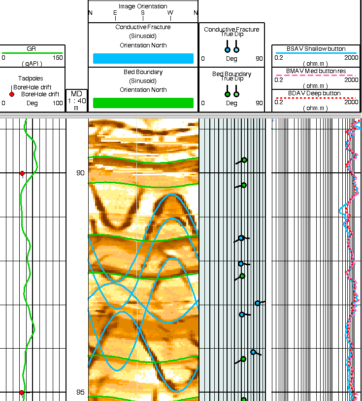
Typical Resistivity-At-Bit (RAB) image log shows gamma ray at
left, resistivity image, dip tadpoles, and 3 resistivity curves
on the right. This image illustrate open fractures (with blue
traces) cross-cutting bedding (in green).
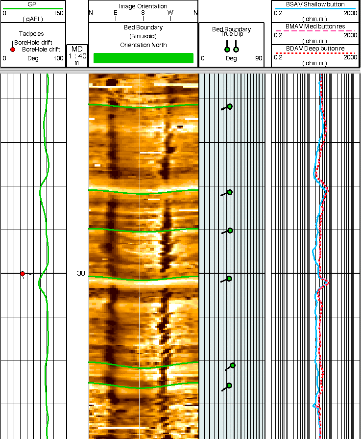
This is an RAB image of an induced fracture )borehole breakout),
not a natural fracture. Induced fractures run parallel to the
borehole axis. Natural fractures almost always cross the borehole.
Fracture
Identification From Acoustic Image Logs
The acoustic
image log (borehole televiewer) is similar in appearance to a
resistivity image log (formation micro-scanner),
but uses an ultrasonic derived, directionally oriented,
360 degree view of the borehole wall.
Such an image, created by
a conventional televiewer, has sufficient resolution to see major
fracture systems in good hole conditions. The hole must be round,
smooth, and filled with light weight mud to get really good images.
The tool must be well centered. These requirements are not met
in most fractured zones, but logs are still run for fracture identification
and they are useful in many cases. Trade names for these tools
are not as well known as others: CBIL (pronounced Cybill) stands
for Continuous Borehole Image Log and UBI for Ultrasonic Borehole
Imager. Versions of these tools are also used for cement evaluation
in cased holes.
The
televiewer log of the wellbore is a representation of the amount
of acoustic energy received at the transducers, which is dependent
upon rock impedance, wall roughness, wellbore fluid attenuation,
and hole geometry. For example, a smooth surface reflects better
than a rough surface, a hard one better than a soft one. A surface
perpendicular to the transducers reflects better than one that
is skewed. Therefore, any irregularities such as fractures, vugs
and irregular porosity will reduce the amplitude of the reflected
signal.
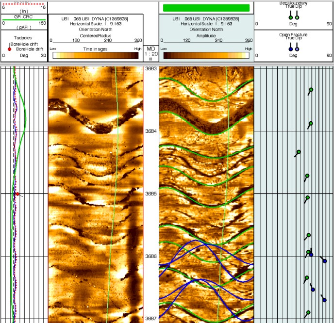
Acoustic Image log with travel time (detailed borehole radius) at
left and amplitude (acoustic impedance) on the right. Fractures show
up as black sinusoid shapes on both images.
Comparison of resistivity image
log (left) and ultrasonic image log in the same borehole. The higher
spatial resolution and the higher dynamic range of the resistivity
image is clear. Black colour represents low acoustic impedance on
CBIL/ UBI, or low resistivity on FMI, in this case representing
fractures (near vertical) or shale beds (near horizontal).
Older acoustic televiewer log (left) and interpretation
image (right)
The
resolution of the tool allows us to determine events of about
10 mm in width. Fractures are often accentuated in the wellbore
by the drilling process, which breaks out the fracture on both
sides of the opening. If it were not for this breakout, most fractures
would not be seen by the televiewer as their width is commonly
less than 1 mm. An example of an actual image from an older televiewer
log, and an interpretive sketch with artificially enhanced resolution. The formation microscanner is much more
sensitive to fractures than the televiewer. The electrical conductivity
of the fluid in the fracture is 1000 or more times higher than
the surrounding rock, compared to about 4 times for acoustic televiewer
signals.
In
addition to the amplitude image, the travel time image is also
recorded on modern logs. This is the travel time from tool to
wellbore wall and back to the detector through the mud. This image
is effectively an acoustic caliper log, and is used to locate
breakouts.
Considerable
research is being conducted to enhance the televiewer images,
using both arrival time and amplitude of the sound waves, plus
computer methods for image enhancement, especially edge enhancement
to resolve fractures and bed boundaries. Modern televiewer logs
can be used effectively in more rugged boreholes than older versions
because of the new processing techniques. Be aware of the age
of the log before you start your analysis.
Since
the televiewer image is oriented to magnetic north, we can determine
the dip direction of a fracture or bedding plane from the azimuth
of the troughs of the sinusoid. The dip angle can be calculated
from the same equation as given for the microscanner.
CAUTION:
The direction scale on the top of the image varies between service
companies. One uses a scale with North in the center of the image
(same as for FMS and FMI), another puts South in the center.
 Here
is a televiewer and core photo of the same fracture.
The sinusoidal shape of the fracture trace is very obvious. In
this image, South is in the center of the track and the fracture
is oriented N 70 E, with a thinner, steeper fracture at N 45 W. Here
is a televiewer and core photo of the same fracture.
The sinusoidal shape of the fracture trace is very obvious. In
this image, South is in the center of the track and the fracture
is oriented N 70 E, with a thinner, steeper fracture at N 45 W.
 Core photo (left) and televiewer image (right) of fractured
interval Core photo (left) and televiewer image (right) of fractured
interval
Fracture
identification is easiest when several detection methods are combined.
This is illustrated in Figures 28.31 and 28.32, where sonic variable
intensity and televiewer images are used. If density of the rock
is also measured, numerous elastic properties of the rock can
be derived, which are useful in hydraulic fracture design and
sanding studies.
Wavetrain and televiewer image with minor fracturing
The
televiewer has a few advantages over the formation microscanner.
These are the ability to see 360 degree image of the borehole,
no need for pad contact, ease of use in oil base muds, high resolution
acoustic caliper, and better steep bed definition due to shallow
investigation. The microscanner has better resolution in rough
hole and has higher dynamic range due to using resistivity contrast
instead of acoustic impedance contrast.
direction at right angles to this
axis. On real, logs check heading carefully, as travel time and
amplitude images can be interchanged in position, and North may be
on the right or the middle of the track.
A
resistivity image log has about 10 times the spatial resolution of an
acoustic image log
and 500 times the amplitude resolution, due to the difference
in contrast between the resistivity and acoustic impedance ranges
measured by the respective tools.
Determining Fracture
DIP and Orientation
Fractures
or bedding planes can be identified by connecting the linear features
to form a sinusoid on the image. The sinusoid can be analyzed
to find the angle of dip:
1:
Angle of Dip = Arctan (Y / D)
Where:
Y = peak to peak distance of the sinusoid (millimeters)
D = hole diameter (millimeters)
Since
Y is measured on a plot or CRT, it must be transformed into actual
wellbore distance by multiplying the measured distance by the
plot scale. Note also that near vertical fractures will appear
near vertical on the plot and do not form sinusoids.
Fracture orientation is determined by the azimuth of the
sinusoid troughs, read from the direction scale at the top of
the image. If image logs are not available, there are other
techniques that might be helpful in estimating the orientation
od fractures, described below.
When formation pressure is isotropic (equal
in all directions), the tectonic stress is zero and Pfrx equals
Pfry. In this situation, the borehole is round and spalling of
the formation is either non-existent or equal in all directions.
In stressed regions, such as in the Rocky Mountains, the borehole
will erode to an oval shape. The minimum diameter shows the direction
of maximum stress and the maximum diameter shows the direction
of minimum stress..
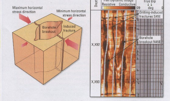
Borehole shape indicates stress direction –
maximum stress in direction of minimum hole
diameter. Formation microscanner and dipmeters have oriented caliper data.
Many
modern logs have an X and Y axis caliper, but not all of them
are oriented to true north. When directional data is recorded,
as with dipmeters and many modern resistivity tools, the X and
Y orientations are known, Statistical plots are helpful in choosing
the dominant direction).
Borehole diameter indicates stress direction -
this example is from India where the minimum
stress direction
is NE - SW.
 A
hydraulic fracture will usually penetrate the formation in a plane
normal to minimum stress, or parallel to the plane of maximum
stress. Any stress anisotropy (tectonic stress) will cause the
fracture to be other than vertical. A
hydraulic fracture will usually penetrate the formation in a plane
normal to minimum stress, or parallel to the plane of maximum
stress. Any stress anisotropy (tectonic stress) will cause the
fracture to be other than vertical.
Natural
fractures take the same directions as hydraulic fractures, indicated
again by the borehole shape. In addition, the high angle dips
seen on an open hole dipmeter or image log, will also indicate this preferential
direction. Since most hydraulic fracture jobs are run in casing,
it is not possible to run a dipmeter or caliper survey to find
the orientation of a hydraulic fracture. The preferential direction
can be predicted from previous open hole data. Dipmeter and caliper
data can be displayed on rose diagrams to illustrate preferential
directions.
If
an azimuthal gamma ray log existed, the fracture orientation could
be located by a tracer survey. I am not aware that such a tool
exists, but it would not be difficult to design one..
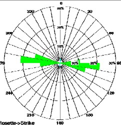
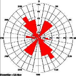
Azimuth frequency (rose diagram) plots show direction of
dips seen on dipmeter and image logs. When steep dips caused by
fractures are isolated from lower angle bedding dips, the
direction of maximum stress xan be determined. In this case, the
direction is N30E.
Stress
direction is not constant over geological time scales. Differences
in the direction of induced fractures (present day stress
direction), open fractures (some time ago), healed fractures (older
than open fractures), and small faults (could be any age) will help
to show the stress history of a region. An example log and rose
diagrams are shown below.
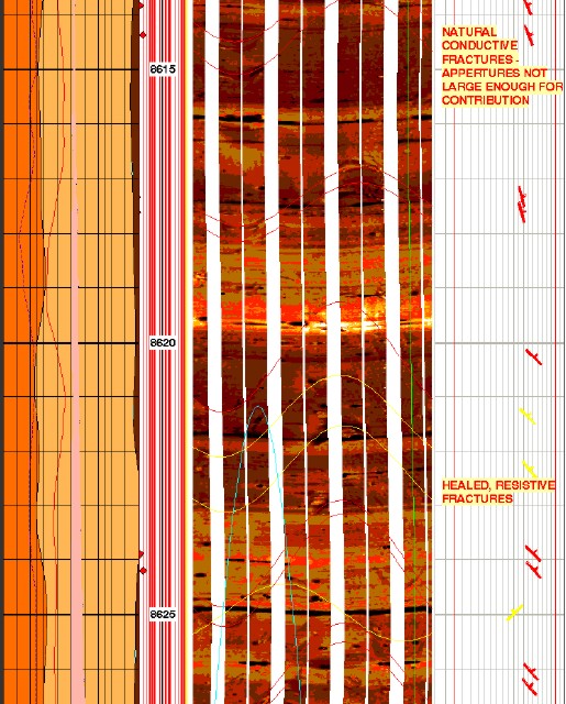
Image log in fractured reservoir: gamma ray (left track, shaded
red), image track (middle) with open fractures (red sine waves and
healed fractures (yellow sine waves), dip track (right) shows red
amd yellow dip angle and azimuth. There are no induced fractures in
this short interval. Bedding planes are near horizontal. Imagine
trying to locate these steep dips without the aid of a computer.
.
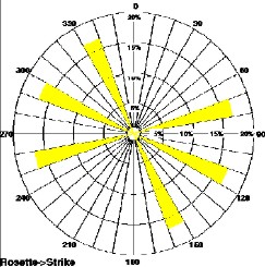
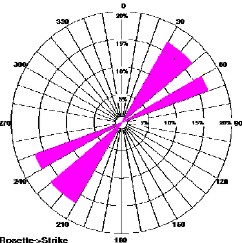
Induced fractures (top left) show current stress direction. Open
fractures (top right) show stress direction when fractures were
created, healed fractures (lower left) show different direction at
an earlier phase in geological time, and micro faults (lower right)
shows another stress regime was present when the faults occurred.
The
newest dipole shear sonic log is also an azimuthal tool with dipole
sources set at 90 degrees to each other. The example below shows the shear images for the X and Y directions. This
log can be run in open or cased hole.
Dipole shear image log shows directional stress
- the Fast Direction is centered on
90 degrees (east - west) which
is also the maximum stress direction.
|