|
 Water Resistivity
TRANSFORMS
Water Resistivity
TRANSFORMS
Water resistivity, salinity, and temperature are
related to each other with various models, described on this
page. Estimating temperature is covered in the next Section
of this Chapter.
Water Resistivity from Salinity
AT ANY TEMPERATURE
Crain's Model is used to convert a lab measured salinity
to a formation water resistivity (RW) at any specific temperature (FT) in degrees Fahrenheit.
The result is abbreviated as RW@FT
throughout this Handbook. You can use equation 5 to convert a
salinity to any arbitrary temperature, for example 75F or 77F
(roughly 25C) to find the resistivity at laboratory conditions.
1: FT = SUFT + (BHT - SUFT) / BHTDEP * DEPTH
2: IF LOGUNITS$ = "METRIC"
3: THEN FT1 = 9 / 5 * FT + 32
4: OTHERWISE FT1 = FT
5: RW@FT = (400000 / FT1 / WS) ^ 0.88
SALINITY FROM WATER RESISTIVITY
Invert Crain's equation to solve for WS given RW at a a specific
temperature FT1.
6:
WS = 400000 / FT1 / ((RW@ET) ^ 1.14)
Where:
BHT = bottom hole temperature (degrees Fahrenheit or Celsius)
BHTDEP = depth at which BHT was measured (feet or meters)
DEPTH = mid-point depth of reservoir (feet or meters)
FT = formation temperature (degrees Fahrenheit or
Celsius)
FT1 = formation temperature (degrees Fahrenheit)
RW@FT = water resistivity at formation temperatures (ohm-m)
SUFT = surface temperature (degrees Fahrenheit or Celsius)
WS = water salinity (ppm NcCl)
COMMENTS:
Use this relation if salinity is known from laboratory measurements
to obtain RW from lab data at any temperature.
NUMERICAL
EXAMPLE:
1. Salinity to water resistivity.
RW@FT = (400000 / 102'F / 20,000 ppm) ^ 0.88 = 0.238 ohm-m @
102'F
(rounded to three significant digits)
2.
Water resistivity to salinity.
WS = 400,000 / 102'F / ((0.250 ohm-m) ^ 1.14) = 19,000 ppm NaCl
(rounded to three significant digits)
Water Resistivity from Salinity
at Lab Temperature
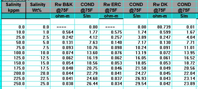
These models generate RW at laboratory temperature of 75F or 25C.
Crain's Method (1974)
1: RW@75F = (400000 / 75 / WS) ^ 0.88
Bateman and Konen Method (1977)
2: RW@75F = 0.0123 + (3647.5 / WS^0.955)
Kennedy's Method (2015)
3: RW@75F = 1 / (24.30853 - 0.0364 *
(0.1 * WS - 29.46515957) - 0.02922 * (0.1 * WS - 29.46515957)^2)
SALINITY FROM WATER RESISTIVITY
Crain's Method (1974)
4:
WS = 400000 / 75 / ((RW@75) ^ 1.14)
Baker Atlas Method (2002)
5: WS = 10 ^ ((3.562 - (Log (RW@75
- 0.0123))) / 0.955)
COMMENTS:
For all
practical purposes, the three models give the same RW value (see
Graph 1 below). There are minor differences above 150,000 ppm NaCl
which can only be seen when water resistivity is converted to water
conductivity (see Graph 2 below).
The effect on water saturation (SW%) is not very significant (+/-
0.5% SW at low SW, +/- 2% SW at high SW, at 200,000 ppm NaCl).
The 10 significant digits used in the Kennedy equation give a false
sense of accuracy that is not warranted.
Dpwnload this spreadsheet:
SPR-08 META/LOG WATER SALINITY (WS) CALCULATOR
Calculate water salinity (WS),
3 methods
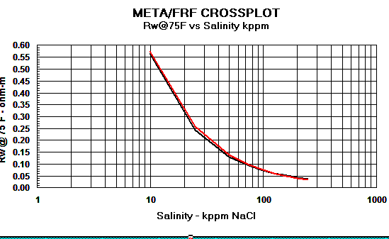
Graph 1:
Rw Models - Red line = Crain, Black line
= Bateman and Konen, Blue line = Kennedy
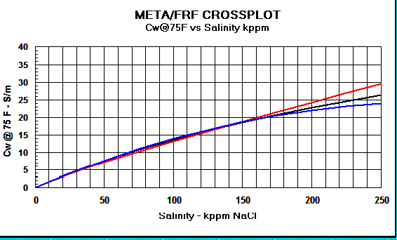
Graph 2:
Cw Models - Red
line = Crain, Black line = Bateman and Konen, Blue line =
Kennedy.
The differences above 150,000 ppm NaCl have little impact on water
saturation.
NUMERICAL
EXAMPLE:
ADJUSTING RW TO FORMATION TEMPERATURE - ARP'S EQUATION
ALSO convert RW @ any temperature to any
other temperature
Water resistivity (RW) data can be found in RW catalogs, drill stem
test and production test reports, and water chemistry reports from a
laboratory. The RW is recorded at a temperature (SUFT) that differs
from the formation temperature (FT) where the log analysis is to be
perforned, so an adjustment is needed. You may already have an RW
value at a particular depth and temperature and want to adjust it to
a different depth and temperature. The math in this Section performs
these tasks..
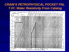
Water catalogues published by your local well logging society
or similar catalogues created by searching in-house data bases
are a necessary tool for well log analysis.
A sample is shown below.
A sample of RW data from a water resistivity catalog, data is tabulated and also
posted on
a map, and is based on a standard temperature of 25 degrees Celsius
(77 degrees Fahrenheit).
 Water
resistivity values in a catalog or a water analysis report are recorded at a standard
temperature, usually 75F or 77F (25C). Since water resistivity varies
inversely with temperature, the catalog values must be
transformed to a new value representing water resistivity at
formation temperature (RW@FT) -- see
next Section. Water
resistivity values in a catalog or a water analysis report are recorded at a standard
temperature, usually 75F or 77F (25C). Since water resistivity varies
inversely with temperature, the catalog values must be
transformed to a new value representing water resistivity at
formation temperature (RW@FT) -- see
next Section.
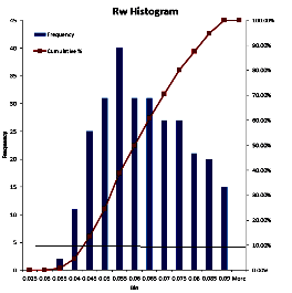
To use data from a water catalogue, it is usually necessary to
do a little filtering. Nearly everything that can go wrong will
raise the RW value recorded in the catalogue. Usually the
minimum value from nearby offset wells is the best choice. It
may be useful to gather all the values for the reservoir for a
radius of 3 to 6 miles (5 to 10 Km) and prepare a histogram. On
the histogram, find the point that represents the lower decile
(10% of the data values are less than this value). Take the
average of the data in this decile. You may want to eliminate
obvious "impossible" values before you make the histogram.
The
following relationships are needed to manipulate water resistivity
data prior to calculations of water saturation.
1. Arps Method (1953)
1:
FT = SUFT + (BHT - SUFT) / BHTDEP * DEPTH
2: KT1 = 6.8 for English units
KT1 = 21.5 for Metric units
3: RW@FT = RW@TRW * (TRW + KT1) / (FT +
KT1)
4: RMF@FT = RMF@TRW * (TRW +
KT1) / (FT + KT1)
5: RMC@FT = RMC@STRW + (TRW * KT1) / (FT + KT1)
Where:
SUFT = surface temperature for temperature gradient
(degrees Fahrenheit or Celsius)
BHT = bottom hole temperature (degrees Fahrenheit or Celsius)
BHTDEP = depth at which BHT was measured (feet or meters)
DEPTH = mid-point depth of reservoir (feet or meters)
FT = formation temperature (degrees Fahrenheit or Celsius)
RMC@FT = mud cake resistivity at formation temperature (ohm-m)
RMC@TRW = mud cake resistivity at surface temperature (ohm-m)
RMF@FT = mud filtrate resistivity at formation temperature (ohm-m)
RMF@TRW = mud filtrate resistivity at surface temperature (ohm-m)
RW@FT = water resistivity at formation temperatures (ohm-m)
RW@TRW = water resistivity at surface temperature (ohm-m)
TRW = temperature at which water was measured (degrees Fahrenheit or Celsius)
2. Hilchie Model (1984) ALL temperatures in Fahrenheit.
6: KT1 = 10^ ( --0.340396 * log(RW@TRW)
+ 0.641427)
7:
FT1 = SUFT + (BHT - SUFT) / BHTDEP * DEPTH
8: RW@FT = RW@TRW * (TRW + KT1) / (FT1 +
KT1)
9: RMF@FT = RMF@TRW * (TRW +
KT1) / (FT1 + KT1)
10: RMC@FT = RMC@STRW + (TRW * KT1) / (FT1 + KT1)
Where:
FT1 = formation temperature (degrees Fahrenheit ONLY)
COMMENTS:
Use
these relations when RW@TRW
is known from measured data. This transformation can be made on
the chart below. The Hilchie model accounts for the slight
curvature at low and high temperatures on the chart, but Arps model
is quite sufficient for practical petrophysics.
NUMERICAL
EXAMPLE:
1. Water resistivity at formation temperature.
English units example:
RW@FT = (0.32 ohm-m @ 77'F) * (77 + 6.8) / (102 + 6.8) = 0.25
ohm @ 102'F
Metric
units example:
RW@FT = (0.32 ohm-m @ 25'C) * (25 + 21.5) / (39 + 21.5) = 0.25
ohm-m @ 39'C
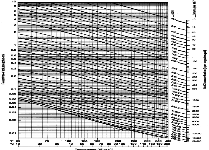
Schlumberger Chart GEN-9: Water resistivity - Temperature - Salinity relationships
|