Igneous and Metamorphic Basics

Medium temperature geothermal projects are often placed in sedimentary rocks, where log analysis methods and rock properties are reasonably well understood. High temperature geothermal is more common in igneous and metamorphic rocks. These are more difficult for petrophysicists to analyze as the physical properties are more variable than those for sedimentary minerals.

Further, igneous and metamorphic rocks are often described by a rock-type name and not by their mineral content. Since logs respond to minerals and not rock-types, an extra step is required to generate rock-types from the mineral components.

This article describes the rock properties as seen by well logs, and the mineral composition of the common rock-types. The objective is to provide the data needed so that you can use your favourite multi-mineral model to resolve the mineralogy of a potential geothermal reservoir in non-sedimentary settings.

Metamorphic rock classification
Metamorphic rocks are conventional sedimentary rocks that have been exposed to high heat and pressure. There are several types of metamorphism: contact, regional, hydrothermal, or fault zone friction, Changes that occur during metamorphism are re-crystallization, neomorphism in which new minerals are created from the original, and metamorphism in which new minerals are created by gaining or losing chemical elements.

Specific sedimentary rocks become specific metamorphic rocks, as shown below:
  Sandstone è Quartzite
  Limestone OR Dolomite è Marble
  Basalt è Schist OR Amphibolite
  Shale è Slate
  Granite OR Rhyolite è Schist
 

These names are familiar to most geologists, but not to many engineers and log analysts who grew up in a sedimentary world.
 

METAMORPHIC ROCK PROPERTIES
The petrophysical properties of metamorphic rocks are often similar to their pre-metamorphic sedimentary counterparts as long as different minerals have not formed. Standard 2- and 3-mineral models, or probabilistic multi-mineral models, are used to calculate lithology. The density neutron complex lithology model is used to calculate porosity when data and borehole conditions permit. Sonic neutron crossplot models can be used as an alternate when needed.

All the algorithms needed are coded in most petrophysical software packages. For explanations of the math, see Reference 1. See Table 1 at the end of this article for a list of matrix properties for metamorphic rocks.

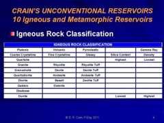
Igneous rock classification
Most people think of granite or lava flows when igneous rocks are mentioned If only it was that simple. There are many variations in rock properties and rock types to take into account during a petrophysical analysis. The mineral and porosity models needed are the same as noted earlier for metamorphic rocks It is more challenging because geologists describe rock-types, which are variable mixtures of minerals, while logs respond only to minerals and not rock-types. We will show how to fix that later on in this article.

Igneous rocks are classified in several ways – by composition, texture, and method of emplacement. The composition (mineral mixture and internal porosity) determines the log response. The texture determines the name used for the mineral mixture, and the method of emplacement determines the texture and internal porosity structure (if any). The same mineral mixture can have more than one name based on its crystal size and method of emplacement.

Intrusive igneous rocks are formed inside the earth. This type cools very slowly and is produced by magma from the interior of the earth. They have large grains, may contain gas pockets, and usually have a high fraction of silicate minerals. Intrusions are called sills when lying roughly horizontal and dikes when near vertical.

Extrusive igneous rocks form on the surface of the earth from lava flows. These cool quickly. They have small grains and contain little to no gas.

Both intrusive and extrusive rocks may contain natural fractures from contraction while cooling, and may have carried non-igneous rocks with them, called xenoliths.

Intrusive rocks may alter the rocks above and below them by metamorphosing (baking) the rock near the intrusion. Extrusives only heat the rock below them, and may not cause much

iteration due to rapid cooling. Extrusives can be buried by later sedimentation, and are difficult to distinguish from intrusives, except by their chemical composition and grain size.

The mineral composition of an igneous rock depends on where and how the rock was formed. Magmas around the world have different mineral make up.

Felsic igneous rocks are light in color and are mostly made up of feldspars and silicates. Common minerals found in felsic rock include quartz, plagioclase, feldspar, potassium feldspar (orthoclase), and muscovite. They may contain up to 15% mafic mineral crystals and have a low density.

Mafic igneous rocks are dark colored and consist mainly of magnesium and iron. Common minerals found in mafic rocks include olivine, pyroxene, amphibole, and biotite. They contain about 46-85% mafic mineral crystals and have a high density. Ultramafic igneous rocks are very dark colored and contain higher amounts of the same common minerals as mafic rocks, about 86-100% mafic mineral crystals.

Intermediate igneous rocks are between light and dark colored. They share minerals with both felsic and mafic rocks. They contain 15 to 45% mafic minerals.

Plutonic and volcanic rocks generally have very low porosity and permeability. Natural fractures may enhance porosity by allowing solution of feldspar grains.

Tuffs and tuffaceous rocks have high total porosity because of vugs or vesicles in a glassy matrix. This is most common in pyroclastic deposits. Interparticle porosity may also exist. Some effort has to be made to separate ineffective microporosity from the total porosity. Pumice (a form of tuff) has enough ineffective porosity to allow the rock to float on water! When other minerals fill the vesicles by precipitation, the tuff is called a zeolite. 
 

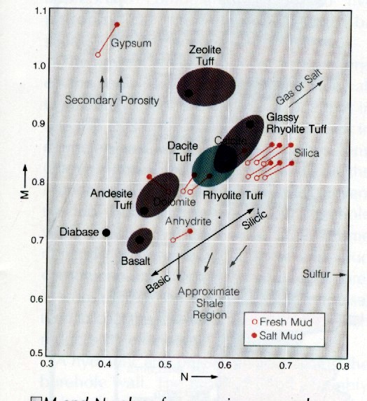
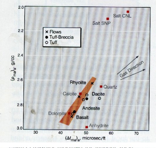
For quick-look identification of igneous rocks, crossplots have been widely used for many years. Before the advent of the PE curve, crossplots using neutron, sonic and density were the best bet. Some prior calculations are required. Matrix density (DENSma), sonic matrix travel time (DTCma), lithology factors Mlith and Nlith must be derived. With the PE curve, a lithology factor called Plith can be added, as well as Uma, the matrix capture cross section. Examples are shown below.

DENSma vs DTCma Crossplot

Mlith vs Nlith Crossplot

Igneous MINERAL properties
Most igneous rocks are described by their rock-type and not by their mineral composition. For example, granite is a rock-type composed of the minerals quartz, feldspar, and plagioclase. Logs respond to the mineral mixture, not the rock-type. Once the mineral fractions are derived by a suitable log analysis model, a second step is needed to convert the minerals to rock-types.

Properties for individual minerals are better known and less variable than rock-type values. It is more accurate to use a mineral model than a rock-type model. Here are the mineral properties that can be used in the various multi-mineral log analysis models. These are the same values that might be used in a sedimentary rock sequence, sorted to reflect the common constituents of igneous rocks.

Sometimes a mineral is determined by triggers based on their specific log responses. For example, where basalt beds are interspersed between conventional granite or quartzite, it is easy to use the PE or density logs to trigger 100% basalt, leaving the remaining minerals to be defined by a two or three mineral model. 

CONVERTING minerals TO ROCK-TYPES
After determining the mineral composition, the rock-type can be estimated from a near-fit to the mineral composition shown in the table below.

This table is based on the illustration given below, courtesy of Schlumberger.

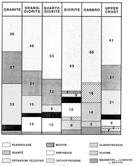
Typical mineral composition of igneous rocks – use as a guide to convert minerals to rock-types.

Since a typical log suite can solve for 3 or 4 minerals at best, you need to choose the dominant minerals and zone your work carefully. If you have additional useful log curves, you might try for more minerals or set up several 4 mineral models in a probabilistic solution. A good core or sample description will help you choose a reasonable mineral suite.
 

eXAMPLe #1 - METAMORPHIC SAND / GRANITE
Here is a granite/metamorphic example from Indonesia. The reservoir has a porous granite at the base, metamorphic sandstone above, topped by conventional sandstone. Porosity is moderately low throughout but the gas column is continuous. Interbedded shales (schist or gneiss in the metamorphic interval) are present but do not act as barriers to vertical flow.

In this case, the mineralogy was calibrated by quantitative sample descriptions, which in turn were keyed to raw log response to minimize cavings and depth control issues. Porosity and water saturation were derived from conventional log analysis methods. The reservoir is naturally fractured and a fracture intensity curve was generated from anomalies on the open hole logs. This was compared to the fracture intensity from resistivity micro image log data.

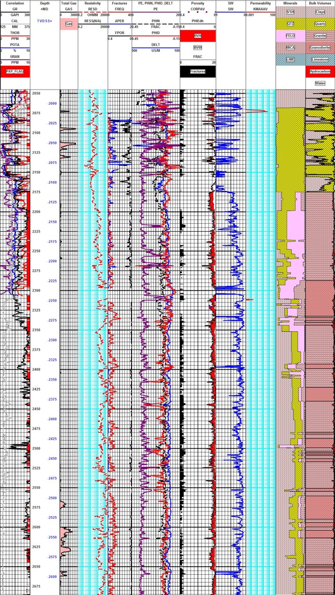
Metamorphic / Granite example with spectral GR (Track 1), total gas (Track 2), resistivity (Track 3), fracture aperture, fracture intensity, fracture porosity (from FMI processing, Track 4), density, neutron, PE (Track 5), log analysis porosity (Track 6), water saturation (Track 7), core permeability (Track 8), quantitative sample description (Track 9), calculated lithology (Track 10).

Compare fracture intensity from log anomalies (black shaded curve in porosity track with fracture intensity from FMI (red curve, track 4). Best gas production in granite is confirmed by gas show on gas log and by production logging in open hole. Sample descriptions show minerals as seen in microscope (quartz, feldspar, mica) to nearest 5%. Log analysis lithology show rock type, not minerals (quartz, granite, granodiorite). The sands and shale immediately above the granite are metamorphosed, visible in samples, but there is little effect on log properties except for low clay bound water on neutron and density logs in the shale/slate. Some wells had limestone marble in the metamorphosed interval.

eXAMPLe #2 - FRACTURED GRANITE WITH POROSITY
Most people forget that there are many unconventional reservoirs in the world, including igneous, metamorphic, and volcanic rocks. Granite reservoirs are prolific in Viet Nam, Libya, and Indonesia. Lesser known granite reservoirs exist in Venezuela, United States, Russia, and elsewhere. Indonesia is blessed with a combination sedimentary, metamorphic, and granite reservoir with a single gas leg. Japan boasts a variety of volcanic reservoirs.

This example is from the Bach Ho (White Tiger) Field in Viet Nam.

Log analysis in these reservoirs requires good geological input as to mineralogy, oil or gas shows, and porosity. A good coring and sample description program is essential, and production tests are essential. The analyst often has to separate ineffective (disconnected vugs) from effective porosity and account for fracture porosity and permeability. All the usual mineral identification crossplots are useful but the mineral mix may be very different than normal reservoirs. Many such reservoirs seem to have no water zone and most have unusual electrical properties (A, M, N), so capillary pressure data is usually needed to calibrate water saturation.

Ternary Diagram for Granite 

In the example below, the granitic mineral assemblage was defined by the ternary diagram at right. The three minerals (quartz, feldspar, and plagioclase) were computed from a modified Mlith vs Nlith model, in which PE was substituted for PHIN in the Nlith equation. If data fell too far outside the triangle, mica was exchanged for the quartz.

Three rock types, granite, diorite, and monzonite, were derived from the three minerals. A trigger was set to detect basalt intrusions. A sample crossplot below shows how the lithology model effectively separates the minerals.

Mlith vs Plith crossplot for granite (micaceous data excluded)

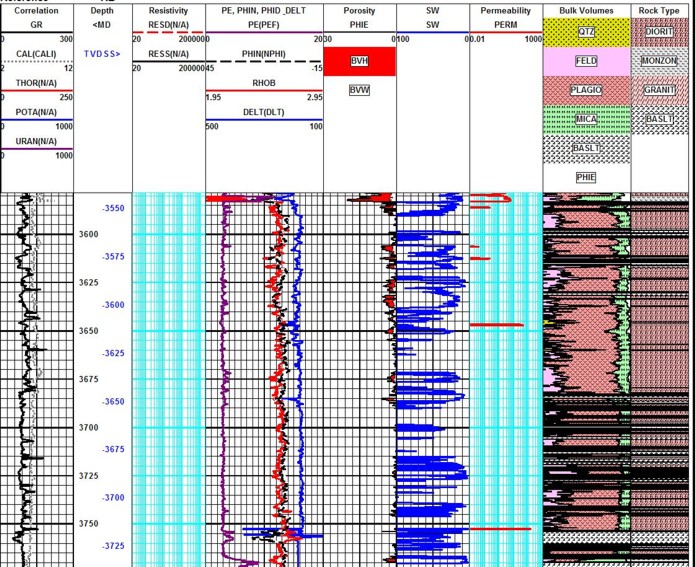
In this fractured granite example, raw data curves are shown in Tracks 1, 2, and 3 with effective porosity, water saturation, and matrix permeability in Tracks 4, 5, and 6. The mineral model calculated from the log analysis is in Track 7 and the rock type model calculated from the minerals using the ternary diagram is in Track 8. Basalt was triggered from high density or high PE or both.

A sample of the log analysis plot is shown above. The average porosity from core and logs is only 0.018 (1.8%) and matrix permeability is only 0.05 md. However, solution porosity related to fractures can reach 17% and permeability can easily reach higher than several Darcies. Customized formulae were devised to estimate these properties from logs, based on core and test data. My colleague Bill Clow devised most of the methods used on this project.

Fracture porosity from resistivity micro scanner logs was also computed where available to help control the open hole work. A black and white resistivity image log below shows some of the fractures. Both high and low angle fractures co-exist.

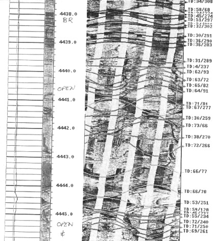
Resistivity micro scanner image in granite reservoir

It is clear that non-conventional reservoirs may need some extra effort, customized models, and unique presentations. Everything you need to develop these techniques can be found elsewhere in this Handbook. The mineral properties need to be chosen carefully, but the mathematical models don't change too much.