|
 POTASH basicS
Potash
refers to potassium compounds and potassium-bearing minerals,
the most common being potassium chloride. The distinguishing
characteristic of potash minerals on well logs is their
relatively high radioactivity, due to the potassium-40
isorope, and their relatively low density compared to other
common sedimentary rocks.
The term
"potash" comes from the old method of making potassium carbonate by leaching wood ashes and evaporating the solution in
large iron pots, leaving a white residue called "pot ash".
Later, "potash" became the term widely applied to naturally
occurring potassium salts and the commercial product derived
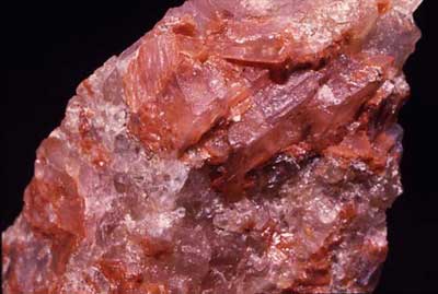
from them. The main potash salts are sylvite, Carnallite,
langbeinite, and polyhalite, mixed in varying concentrations with halite (rock salt). The main use of potash is as fertilizer.
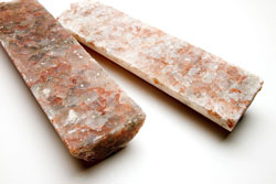 Sylvinite is the most important ore for the production of potash
in North America. It is a mechanical mixture of sylvite (KCl, or
potassium chloride) and halite (NaCl, or sodium chloride). Most
Canadian operations mine sylvinite with proportions of about 31% KCl
and 66% NaCl with the balance being insoluble clays, anhydrite, and
in some locations carnallite. Sylvinite is the most important ore for the production of potash
in North America. It is a mechanical mixture of sylvite (KCl, or
potassium chloride) and halite (NaCl, or sodium chloride). Most
Canadian operations mine sylvinite with proportions of about 31% KCl
and 66% NaCl with the balance being insoluble clays, anhydrite, and
in some locations carnallite.
Sylvinite ores are beneficiated by
flotation, dissolution,-recrystallization, "heavies" separations,
or combinations of these processes.
 The major source of potash
in the world is from
the Devonian Prairie Evaporite Formation in Saskatchewan, which
provides 11 million tons per year. Russia is second at 6.9 million
and the USA (mostly from New Mexico) at 1.2 million tons per year. A
dozen other countries in Europe, Middle East, and South America
produce potash from evaporite deposits. The major source of potash
in the world is from
the Devonian Prairie Evaporite Formation in Saskatchewan, which
provides 11 million tons per year. Russia is second at 6.9 million
and the USA (mostly from New Mexico) at 1.2 million tons per year. A
dozen other countries in Europe, Middle East, and South America
produce potash from evaporite deposits.
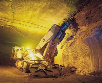
Potash can be mined mechanically
by underground machinery or by solution mining using ambient or
warmed water. Halite (salt) for human use or road de-icing
can be mined the same ways. Potash ores contain halite as well, so
the by-product of potash extraction is road salt. In earlier times,
salt was more valuable per ounce than gold, as it was essential to
human life. A person "worth his salt" was one who contributed his
fair share to the community.
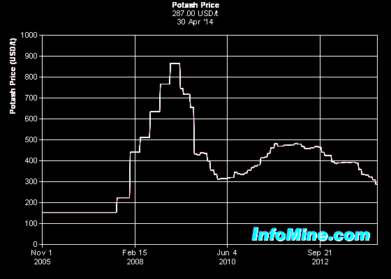 Potash
prices have undergone a flurry of variation since 2005, after many
years of relatively stable values. A perceived shortage of supply
moved the price from around $200 per tonne to nearly $900 per tonne,
falling quickly to the $300 to $500 range. The breakup of the
Russian / Belerus potash cartel in 2012 pushed prices into the $300
per tonne range and by 2014 appeared to be stabilized near this
value. The future is unpredictable. Potash
prices have undergone a flurry of variation since 2005, after many
years of relatively stable values. A perceived shortage of supply
moved the price from around $200 per tonne to nearly $900 per tonne,
falling quickly to the $300 to $500 range. The breakup of the
Russian / Belerus potash cartel in 2012 pushed prices into the $300
per tonne range and by 2014 appeared to be stabilized near this
value. The future is unpredictable.
PROPERTIES OF POTASH Minerals
 Potassium is radioactive so the gamma ray log is used to
identify potash bearing zones. Potash minerals have distinctive
physical properties on other logs, so conventional multi-mineral
models can be used to determine the mineral mixture, just as we
do in carbonates in the oil and gas environment. Potassium is radioactive so the gamma ray log is used to
identify potash bearing zones. Potash minerals have distinctive
physical properties on other logs, so conventional multi-mineral
models can be used to determine the mineral mixture, just as we
do in carbonates in the oil and gas environment.
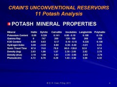
For
consistency, potash ore and fertilizer concentrations are rated
by their equivalent K2O content. Some literature can be
confusing because they rate the ore by its potassium content (K)
or potassium chloride content (KCl), The table below lists the
physical properties of potash minerals, including K and K2O
values. The GR (API units) entry in the table do not seem to
match any known correlation, so some caution is urged.
|
POTASH MINERAL PROPERTIES -- FRESH MUD |
|
Mineral |
PHIN |
DENS |
DTC |
DTC |
PE |
Uma |
Mlith |
Nlith |
Alith |
Klith |
Plith |
GR |
K2O |
K |
Formula |
|
|
Ls |
g/cc |
us/m |
us/ft |
barns |
cu |
frac |
frac |
frac |
frac |
frac |
Gapi |
frac |
frac |
|
|
|
|
|
|
|
|
|
|
|
|
|
|
|
|
|
|
Water |
1.000 |
1.00 |
656 |
200 |
0.10 |
0.10 |
|
|
|
|
|
|
|
|
|
|
|
|
|
|
|
|
|
|
|
|
|
|
|
|
|
|
Halite |
-0.010 |
2.03 |
220 |
67.1 |
4.72 |
9.58 |
1.291 |
0.981 |
1.020 |
1.316 |
4.583 |
0 |
0.000 |
0.000 |
NaCl |
|
Sylvite |
-0.041 |
1.86 |
242 |
73.8 |
8.76 |
16.29 |
1.468 |
1.210 |
0.826 |
1.213 |
10.186 |
953 |
0.630 |
0.524 |
KCl |
|
Carnallite |
0.584 |
1.56 |
256 |
78.0 |
4.29 |
6.69 |
2.178 |
0.743 |
1.346 |
2.932 |
7.661 |
255 |
0.170 |
0.141 |
KMgCl3●6H2O |
|
Langbeinite |
-0.020 |
2.82 |
170 |
52.0 |
3.56 |
10.04 |
0.813 |
0.560 |
1.784 |
1.451 |
1.956 |
342 |
0.226 |
0.188 |
K2SO4Mg2(SO4)2 |
|
Polyhalite |
0.150 |
2.79 |
188 |
57.5 |
4.32 |
12.05 |
0.796 |
0.475 |
2.106 |
1.676 |
2.413 |
235 |
0.155 |
0.130 |
K2SO4Mg(SO4)(Ca(SO4))2●2H2O |
|
Kainite |
0.300 |
2.12 |
213 |
65.0 |
3.50 |
7.42 |
== |
0.625 |
1.600 |
== |
3.125 |
285 |
0.189 |
0.156 |
KMg(SO4)Cl·3H2O |
|
|
|
|
|
|
|
|
|
|
|
|
|
The GR values shown above will vary with tool type and calibration
is performed only at low GR flux (about 200 - 250 API units). Quoted
values for sylvite are >500, 753, 953, 1046. A correlation between
sylvite or K2O content should be done to calibrate a particular tool
type whenever possible. GR values for the other minerals can be
prorated based on their K or K2O content.
Actual sonic travel time in halite and sylvite may be
slightly higher than shown above due to occluded water. The Vp/Vs
ratio for most salts is close to 1.9 so shear travel time is
close to 1.9 times compressional travel time.
The above physical properties are used in the standard 2- and
3-mineral models, simultaneous equation models, and
multi-mineral probabilistic models. Choose the mineral mix to
match the actual mineralogy as described in cores or samples.
Add clay or quartz to account for insolubles and occluded water
if enough independent log curves are available.
REFERENCES:
1. Quantitative Log Evaluation of the Prairie Evaporite
Formation of Saskatchewan
E. R. Crain,
P.Eng., W.B. Anderson,
P.Eng.
Journal of Canadian Petroleum Technology, Quebec City
and Edmonton, Jul- Sep, 1966
 As published, 1966
As written with legible illustrations, 1964
Program for IBM 1620, 1964
2. Defining Evaporite Deposits with Electrical Well Logs
R. P. Alger, E. R. Crain,
P.Eng.
Trans Northern Ohio Geological Society - Second
Symposium on Salt, Cleveland, 1966
3. Potash Redux
E. R. Crain, P.Eng., CWLS InSite, Dec 2010
LOGGING IN POTASH WELLS
The minimum logging program for a potash interval is gamma
ray and a neutrom log. A sonic, density, and PE logs are useful
in assessing accessory minerals. A resistivity log is usually
required elsewhere in the rest of the wellbore so it is usually
run in combinatation with the others. Here are some examples.
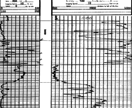
Example of a 1964 gamma ray neutron log from Saskatchewan.
Note the primary GR with 2 backup curves in Track 1. This is
hard to use quantitatively, so an alternative GR dis]lay was
common before the digital era, as shown below.
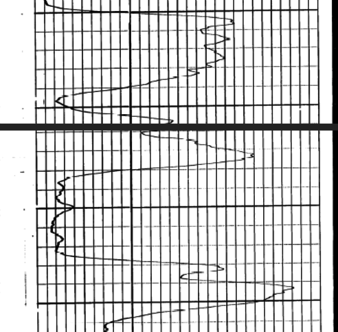 . .
Example of a 1964 3-track gamma ray log presentation,
common before the digital era. GR scale is 0 to 600 API units. Log data values picked from these
logs are used to create a transform relating the log data to
core assay data. An example of such a transform is shown later
on this webpage.
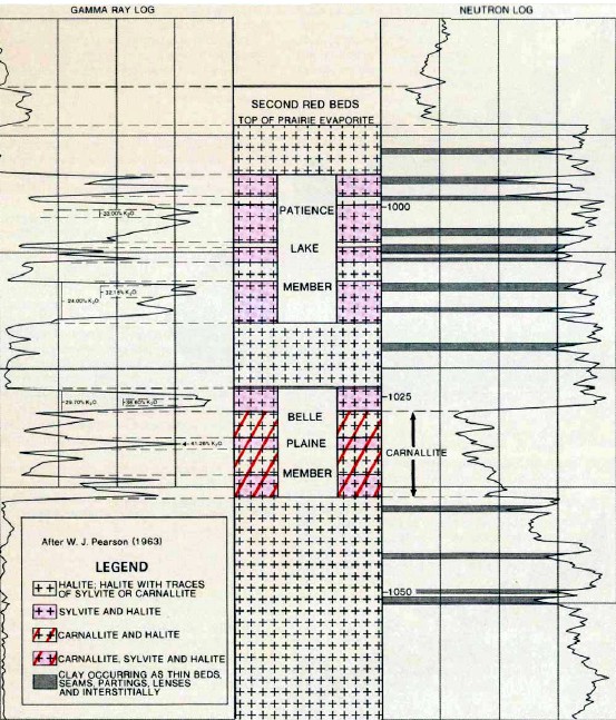
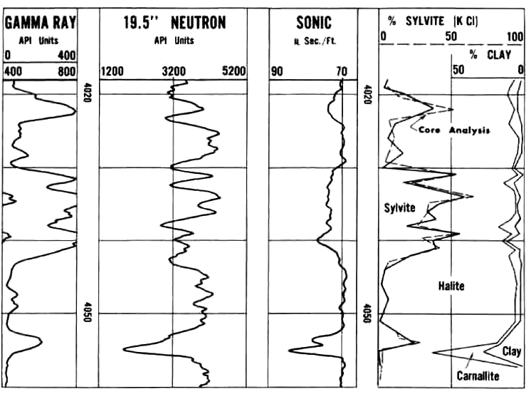
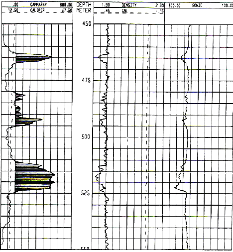
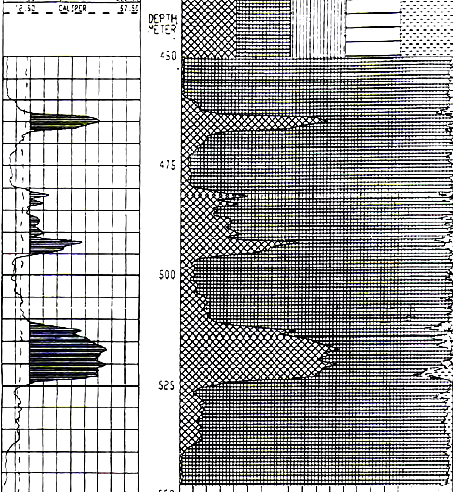
Example gamma ray and neutron log from Saskatchewan showing
halite, sylvite, Carnallite, and clay responses. In the
exploration heyday in Saskatchewan in the 1960's, we presented
the gamma ray across 3 tracks of the log, giving a scale of 0 to
450 or 0 to 600 API units across 7.5 inches of paper. This was
sufficient resolution for accurate evaluation and eliminated the
need for GR backup curves cramped into Track 1.
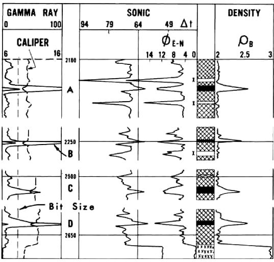
1970's era logs in a potash interval in New Mexico. Visual
analysis is based on review of the four log
curves: GR, sonic, neutron, and density.
POTASH MINERAL IDENTIFICATION FROM CROSSPLOTS
Crossplots of well log data have been used
for many years in the oil, gas, and sedimentary mineral
industries. A number are shown below -- they are not found in
standard service company chartbooks.
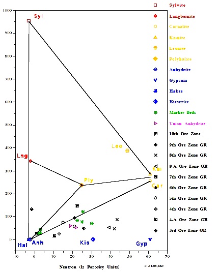
The most useful is a crossplot of gamma ray versus neutron
porosity. Commercial potash ores are anhydrous (no water of
hydration), such as sylvite and langbeinite, so the neutron log
reads near zero. Hydrated potash minerals will have non-zero
neutron response, such as Carnallite, polyhalite, and kainite.
High gamma ray response distinguishes all these minerals from
other zero porosity minerals, such as halite and anhydrite, and
from porous minerals, such as calcite, dolomite and clay.
Potash beds seldom contain pure minerals; usually they are made
of a mixture of one or more potash minerals with halite. Thus
data points will fall on trend lines joining the pure mineral
points. The best examples are the Potash Identification Plots (PID
plots) contained in "Simple Screening Technique for Identifying
Commercial Potash", by Donald G. Hill Ph.D., AAPG,
2019. Here are some examplws.
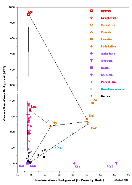
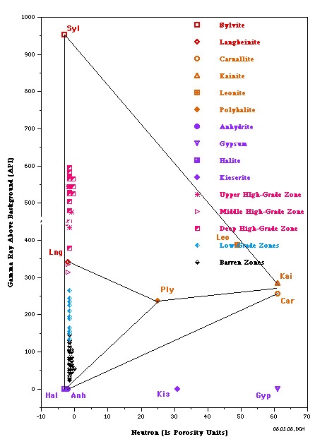
PID Plots for Prairie Evaporite in Saskatchewan (left) and
Windsor Salt jn Nova Scotia (right). Both show data points along
the near vertical Sylvite - Langbeinite - Halite trend line,
indicating commercial grade potash ore. Only the Saskatchewan
example shows some data trending toward the non-commercial
Carnallite data point. Note that the GR scale on the vertical
axis is for a moden logging tool with a linerar response. For
older tools, the Y-axis could be replaced with a K2O axis,
derived from the original Crain non-linerar relationship.
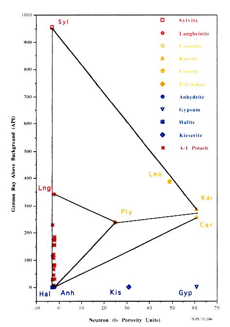
The Michigan Basin example (left) shows only commercial grade
potash ore in this well. The New Mexico example (right) shows
only non-commercial ore in this well.
The following crossplot illustrations were derived from the
well logging literature.
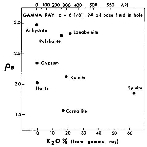
Gamma ray and K2O content versus density crossplot of evaporite minerals
used for mineral identification. Note that the GR scale is
non-linear based on Crain's correlation of 1960's era logs;
modern GR logs are linear beyond 1000 API units and require a
different calibration to K2O content.
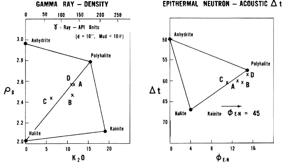
Density versus K2O fs and Sonic versus Neutron Crossplots for some
potash minerals.
POTASH ANALYSIS - OLDER LOGS
 Since
potassium is radioactive, the K2O content can be derived from
gamma ray logs, and this technique has been used since the
1960's. In 1964, I was stationed in Lanigan, Saskatchewan to run
logs in potash exploration wells. While there, I scrounged a
personal tour of the Esterhazy potash mine, then only two years
old. This was the first and only time I have seen geological
structure and stratigraphy from the "inside" of the rock. Truly
amazing! Since
potassium is radioactive, the K2O content can be derived from
gamma ray logs, and this technique has been used since the
1960's. In 1964, I was stationed in Lanigan, Saskatchewan to run
logs in potash exploration wells. While there, I scrounged a
personal tour of the Esterhazy potash mine, then only two years
old. This was the first and only time I have seen geological
structure and stratigraphy from the "inside" of the rock. Truly
amazing!
No direct calibration between GR and K2O had been developed up to that time, so I convinced a
client to let me see his core assay data. After adjusting for
hole size, mud weight, and bed thickness, a reasonable relationship was found,
and was published as "Quantitative Log Evaluation of the Prairie Evaporite
Formation of Saskatchewan" by E. R. Crain and W. B. Anderson,
Journal of Canadian Petroleum Technology, July--September, 1966.
The work was subsequently reprinted in
five other papers by various authors, some included updates as
tool technology evolved. The original GR correlation was
unchanged, widely distributed,
and was the standard for potash analysis from oilfield style
logs run prior to the era of
digital logs in the 1980's. Most analog oil field GR logs were
non-linear above about 300 API units due to dead time in the counting
circuit. These older logs are still available in the well files
and were recently used by Saskatchewan Industry and Resources to
update their potash isopach and ore grade maps.
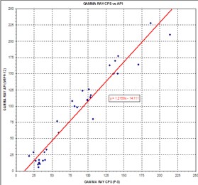
K2O versus Gamma Ray relationship for analog
Schlumberger tools circa 1960 - 1975, run in open hole with oil
based mud. Tools from other service
companies may differ. Correlation between log and core assay
data for specific cases is strongly recommended. Modern gamma
ray logs respond in a more linear fashion and slope may be
different due to more efficient detectors.
|
K2O from GRc |
|
GR API |
K20 |
|
0 |
0.0 |
|
45 |
2.5 |
|
90 |
5.0 |
|
135 |
7.5 |
|
175 |
10.0 |
|
220 |
12.5 |
|
265 |
15.0 |
|
310 |
17.5 |
|
355 |
20.0 |
|
400 |
22.5 |
|
435 |
25.0 |
|
470 |
27.5 |
|
505 |
30.0 |
|
530 |
32.5 |
|
550 |
35.0 |
|
565 |
37.5 |
|
580 |
40.0 |
|
590 |
42.5 |
|
600 |
45.0 |
|
605 |
47.5 |
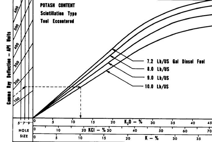
GAMMA RAY BOREHOLE CORRECTIONS
The hole size and mud weight corrections derived from
the data, and embedded in the above chart, were:
1. GRh = GR * (1.0 +.0.05 * (HS - 6.0)) + (320 *
(HS - 6.0)) / (GR + 100.0)
2. GRc = GRh * (1.0 + 0.10 * (WM - 7.2))
Where:
GR = gamma ray log reading (API)
GRc = GR corrected for hole size and mud weight (API)
GRh = GR corrected for hole size (API)
HS = hole size (inches)
WM = mud weight (lb/gal)
POTASH ORE GRADE FROM GAMMA RAY
K2O content was derived from GRc using the lookup table shown at
the right. It is linear up to 400 API units and exponential
thereafter. Values in the table represent a 6 inch borehole
filled with diesel at 7.2 lb/gal. The linear portion of the
lookup table is represented by:
3: IF GRc <= 400
4: THEN K2O = 0.05625 * GRc
5: OTHERWISE Use Lookup Table
The slope in the above equation can be determined by
correlation to core assay data for other hole sizes or other
tool types.
The non-linear relationship must be honoured while
analyzing these older logs for potash. The effect is negligible
for conventional oil field applications. Modern digital tools are linear up
to about 1000 API units so the discussion in this Section does
not apply.
A 1967 paper showed a linear GR relationship up to
650 API units for the McCullough tool, but its use was not
widespread in Canada. That graph showed 600 API units was
equivalent to 45% K2O, identical to my original data, but the
slope of the line at lower GR readings was different. No mud
weight correction was implied but a bed thickness correction
similar to mine was presented.
 In
the analog era, GR logs were calibrated to a secondary standard
based on the API GR test pit in Houston which contained an
artificial radioactive formation defined as 200 API units in an
8 inch borehole filled with 10 lb/gal mud. In
the analog era, GR logs were calibrated to a secondary standard
based on the API GR test pit in Houston which contained an
artificial radioactive formation defined as 200 API units in an
8 inch borehole filled with 10 lb/gal mud.
However, there were
no published borehole size or mud weight correction charts for
the GR log. These effects are large enough to seriously
compromise the correlation.
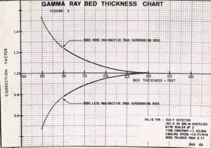
BED THICKNESS ISSUES
Bed thickness corrections are also
needed for beds less than 3 feet thick (1 meter). This is
true even for modern logs. The
chart shown at the right illustrates the importance
of normalizing the GR log for these factors. Unfortunately, my
original data plots for this work were lost in the bowels of a
Schlumberger shredder many years ago - it would have been nice
to recalibrate the work with the power of non-linear regression
in a good statistics package.
 NON-OILFIELD GAMMA RAY TOOLS
Many
potash exploration wells in the USA and elsewhere were logged with
slim hole GR tools intended for uranium work. While they may have
been more linear, they were not usually calibrated to any standard,
suffered from larger borehole effects, and were recorded in counts
per second (cps). Specific correlations to core assay data on a well
by well basis are required for these wells.
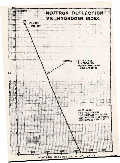
USING ANCIENT NEUTRON LOGS
Due to the water of hydration
associated with Carnallite, the neutron log is very useful for
distinguishing between Carnallite and sylvite. High neutron count
rates mean low hydrogen index, thus sylvite and not Carnallite.
To quantify the relative amounts
of Carnallite and sylvite, the neutron response must be converted to
porosity from count rates using the standard semi-logarithmic
relationship. A typical transform for a 1960's era Schlumberger
tool is shown at the left. Charts for other tools can be found in ancient
service company chart books.
With the advent of the
sidewall neutron log in 1969 and later the compensated neutron log,
this transform was no longer required.
USING SONIC AND DENSITY LOGS
Some wells were logged with sonic
and/or density logs in addition to the neutron log, which also could
be used quantitatively with the GR and neutron to provide a potash
assay based on logs. This was important where core was lost or for
regional exploration when core data, but not the logs, were
proprietary. The logic behind these models is shown below. A later
Section of this article deals with the use of more modern logs.
POTASH ModelS - OLDER LOGS
My original computer program for potash analysis was written for
the IBM 1620 in Regina in 1964. The model was based on four
simultaneous equations that define the response of the available
logs. Although this seems like a long time ago, nothing has changed
except the improved tool accuracy. If you want to analyze the older
log suites, here's how to do it.
The
minerals sought are halite (rock salt), sylvite, Carnallite, and
insolubles or clay. The only logs available on old wells are
resistivity, sonic, neutron, and total gamma ray. The
resistivity is not a helpful discriminator, except as a shale
bed indicator, so it is not used in the simultaneous solution.
These evaporite beds contain potassium and ore grade is measured
in units of potassium oxide (K2O). K20 is obtained from a gamma
ray log, corrected for borehole size and mud weight, using a
non-linear transform derived from core assay data. In middle
aged wells, the density log is also helpful, and in modern wells
the PE curve can be added. Further, the gamma ray response is
linear on modern wells so the transform to K2O is not as
difficult to obtain.
The equations are:
1.00 = Vsalt + Vsylv + Vcarn + Vclay
K20 = 0.00 * Vsalt + 0.63 * Vsylv + 0.17 * Vcarn + 0.05 * Vclay
PHIN = 0.00 * Vsalt + 0.00 * Vsylv + 0.65 * Vcarn + 0.30 * Vclay
DTC = 67 * Vsalt + 74 * Vsylv + 78 * Vcarn + 120 * Vclay
K2O is
obtained, after borehole correcting the GR, from the equations and
lookup table shown
earlier, or from a fresh correlation based on specific data from the
wells under study. Note that the chart and table given earlier are
in percent K2O and this set of equations expects fractional units
for K2O, neutron porosity, and all output volumes. Parameters in the
sonic equation are in usec/ft.
When
solved by algebraic means, these equations become:
1: Vclay = 0.0207 * DTC - 0.23 * K20 - 0.29 * PHIN - 1.3891
2: Vcarn = 1.54 * PHIN - 0.46 * Vclay
3: Vsylv = 1.59 * K20 - 0.41 * PHIN + 0.04 * Vclay
4: Vsalt = 1.00 -
Vclay - Vsylv - Vcarn
These equations were derived with DELT in usec/ft. All constants
will be different if DELT is in us/m.
To
convert from mineral fraction to K2O equivalent (K2O equivalent
is the way potash ores are rated), the final analysis follows:
5: K2Osylv = 0.63 * Vsylv
6: K2Ocarn = 0.17 * Vcarn
7: K2Ototal = K2Osylv + K2Ocarn
EFFECT OF OCCLUDED WATER
If
occluded water (V) is added to the desired results, the equations become:
1.00 = Vwtr + Vsalt + Vsylv + Vcarn + Vclay
Where
Vwtr = PHIN value in pure salt above the zone of interest.
The
occluded water has zero gamma ray emission so the second equation
remains unchanged:
K20 = 0.00 * Vsalt + 0.63 * Vsylv + 0.17 * Vcarn + 0.05 * Vclay
The
porosity is read directly by the neutron log, hence, the third
equation becomes:
PHIN = 1.00 * Vwtr + 0.00 * Vsalt + 0.00 * Vsylv + 0.65 * Vcarn
+ 0.30 * Vclay
The
sonic equation becomes:
DELT = C + 67 * Vsalt + 74 * Vsylv + 78 * Vcarn + 120 * Vclay
Where
C = DELT in salt minus 67 usec/ft.
Reduction
of these equations results in:
8: Vclay = 0.0207 * (DELT - C) - 2.23 * K20 - 0.29 * (PHIN - V) - 1.3891
9: Vcarn = 1.54 * (PHIN - V) - 0.64 * Vclay
10: Vsylv = 1.59 * K20 - 0.41 * (PHIN
- V) - 0.04 * Vclay
11: Vsalt = 1.00 - Vsylv - Vcarn - Vclay
- Vwtr
Conversion
to K20 equivalent remains the same as before. Note that mineral
fractions are in volume fractions. To convert to
weight fraction, one more step is needed. By using the density
of each mineral times the volume fraction, summing these to get
the total rock weight, then dividing each individual weight by
the rock weight, we get weight fraction of each. This allows
comparison to core assay data which are reported in weight
fraction or percent. The same math is used in tar sands and coal
analysis to allow comparison to lab data.
12: WTclay = Vclay * 2.35
13: WTcarn = Vcarn * 1.61
14: WTsylv = Vsylv * 1.98
15: WTsalt = Vsalt * 2.16
16: WTwtr = Vwtr * 1.10
17: WTrock = WTclay + WTcarn + WTsylv + WTsalt +
WTwtr
Note
that the densities in the above equations are the true density
values, not the electron densities used in the original
simultaneous equations.
Mass
fraction or weight percent values are obtained b dividing individual
weights by WTrock. foer example:
18: Wsylv = WTsylv / WTrock
19: Wcarn = WTcarn / WTrock
20: WT%sylv = 100 * Wsylv
21: WT%carn = 100 * Wcarn
Where:
Vxxx = volume fraction of a component
WTxxx = weight of a component (grams)
Wxxx = mass fraction of a component
WT%xxx = weight percent of a component
COMMENTS
These
equations show the use of constraints (Vwtr and C) on the otherwise
linear simultaneous equations. The first set of equations is exactly
determined, and the second set are underdetermined until Vwtr and
C are defined.
If
the density or PE equation were added, then the set would be exactly
determined and the strategy of finding Vwtr and C in the pure salt
bed would not be needed. This work was done in Saskatchewan before
density logs were common, so the density equation was not used
at that time.
POTASH MODELS - MODERN LOGS
With a modern suite of calibrated logs, we can use
conventional multi-mineral models to calculate a potash assay.
With GR, neutron, sonic, density, and PE, we can solve for
halite, sylvite, Carnallite, clay (insolubles or shale
stringers), and water (occluded in many salts as isolated
pores). The potassium curve from a spectral gamma ray log might
also prove useful, if the detector system is linear and does not
saturate. Alternate mineral models are quite possible in other
potash areas of the world.
The mathematical methods are covered in the Lithology Chapters elsewhere
in this Handbook. Matrix rock properties for the minerals were
shown earlier in this article. Water is treated as a "mineral"
so that it can be segregated from the water of hydration in
Carnallite.
Probabilistic analysis methods are also used with modern log
suites. Here, the mineral mixture can be underdetermined,
allowing the program to find the best mix at any particular
depth point.
 The
first step is to correct the gamma ray for borehole and mud
weight effects, using the appropriate service company correction
charts. The other logs seldom need much correction as the potash
is not deep or hot. However, if a water based mud was
used, it will have a high salinity, so a salinity correction for
the neutron log may be required. The
first step is to correct the gamma ray for borehole and mud
weight effects, using the appropriate service company correction
charts. The other logs seldom need much correction as the potash
is not deep or hot. However, if a water based mud was
used, it will have a high salinity, so a salinity correction for
the neutron log may be required.
The second step is to confirm the GR to K2O correlation using
any available potash core assay data. Since modern GR logs are
more linear than older tools, the relationship should be a
relatively straight line and can be extended beyond the
available core data, as shown at the right.
SPECIAL CASES
There are numerous situations which require special
treatment. These include:
1. an incomplete open hole logging suite
2. logs run through casing
3. logs run with GR in counts per second
4. logs run where thin beds predominate
5. combinations of the above.
Incomplete Logging Suite
Here we must include fewer minerals in the model. Isolated
water is easy to ignore, and insoluble clay comes next, although
it is an important economic factor in the extraction process. In
the worst case, we might need to settle for K2O from the gamma
ray and a sylvite / Carnallite discriminator based on the neutron
log. This situation occurs most often when potash geologists are
using logs in wells drilled originally for oil or gas, in which
potash evaluation was not considered as a priority.
Through Casing Logs
The most obvious problem will be to correct the gamma ray log
for casing size and weight, cement sheath thickness, and
borehole fluid weight using service company correction charts.
Where core assay data is available from the well or from
reasonably close offsets, the GR to K2O relationship can be
confirmed. The second problem is usually an incomplete logging
suite, as described above. If a through casing neutron log is
available, scaled or not, a Carnallite flag can be created.
GR in Counts per Second
Many potash wells are drilled as stratigraphic test wells
and are not intended to be completed. They are often drilled as
slim holes and slim hole GR logs must be run. Some of these logs
may be calibrated to the API GR standard; many are not. In any
case the GR to K2O correlation must be established for each tool
type and adjusted if mud weight or borehole size varies between
wells. Bear in mind that the core retrieved from a slim hole is
volumetrically much smaller than full size cores. Variations
between log and core data is expected to be somewhat larger in
slim holes.
Thin Bed Problems
This issue affects all logs used for all purposes, but
can seriously affect potash evaluation in areas where thin beds
predominate. An approach was shown earlier using a bed thickness
correction chart. Another approach is to correlate K2O times
thickness to GR times thickness instead of a direct GR to K2O
transform. This is best suited to hand picked data, as thickness
is not so easily determined automatically in most log analysis
software. The US Geological Survey published an example,
originally developed by Jim Lewis of Intrepid Mining for a New
Mexico case study. The pertinent crossplots from his work are
shown below. The regression has much less scatter on the GR
times thickness plots. This method was originally suggested in a
1967 paper describing the use of McCullough GR logs for potash
evaluation.
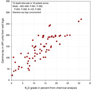
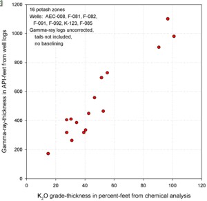
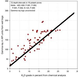
GR in API units vs K20 (left) shows poor correlation due
to thin bed effects. GR-thickness vs K2O-thickness products
(right) correlate much better (regression lines not shown).
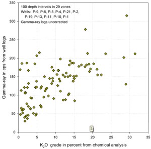
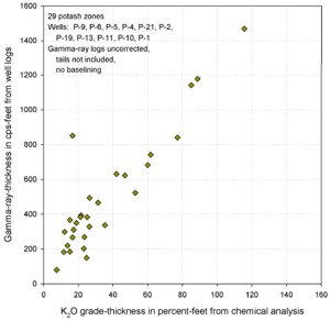
Similar graphs for some USGS GR data in cps show that the GR-thickness
product is a better predictor of potash content than GR by
itself in thinly bedded potash zones..
Combinations of the Above
 It
would be unusual if there were no problems to solve. Logs run in
different areas by a variety of service companies need to be
normalized to some single standard. Borehole and casing effects
need to be handled first. Then normalizing oilfield and strat
hole gamma ray logs can be done by correlating potash beds
between near offset wells. It would be nice if both wells also
had core assay data but this is seldom the case. At right is a
comparison of USGS log picks over 29 potash intervals showing
the regression against the API units for the same zones in the
nearest oilfield well. The equation of the line can be used to
convert all USGS logs to API units in this particular project
area. It
would be unusual if there were no problems to solve. Logs run in
different areas by a variety of service companies need to be
normalized to some single standard. Borehole and casing effects
need to be handled first. Then normalizing oilfield and strat
hole gamma ray logs can be done by correlating potash beds
between near offset wells. It would be nice if both wells also
had core assay data but this is seldom the case. At right is a
comparison of USGS log picks over 29 potash intervals showing
the regression against the API units for the same zones in the
nearest oilfield well. The equation of the line can be used to
convert all USGS logs to API units in this particular project
area.
Ancient GR logs could be rescaled with a non-linear transform
to make them respond similarly to modern logs. Once the
conversion is made, computer analysis is easier and cross
sections look better.
POTASH ANALYSIS EXAMPLES - OLDER LOGS
A sample of computed results from this log analysis
model compared to core data is shown below. The GR was borehole
corrected but no bed thickness corrections were applied.
Example log analysis showing excellent match to core data (circa
1964). Raw data is shown but note the scales are opposite polarity
to normal.
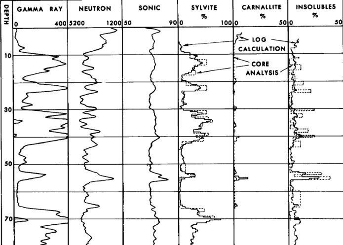
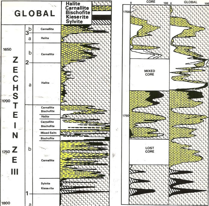
Another Saskatchewan example with sylvite, salt, and clay compared
to core assay, grading to Carnallite near the base, normal log presentations.
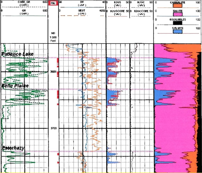
Potash evaluation of 1960's logs with a modern log analysis program.
The core gamma ray (dashed curve, Track 1) reads considerably higher
than the open hole GR log (solid curve). Using Crain's original
non-linear algorithms on the log data, results match core assay data
(see data in K2OS and K2OC tracks). A linear transform would be
needed to calibrate K2O from the core gamma curve.
POTASH ANALYSIS EXAMPLES - OLDER LOGS
1990's example from the Windsor Salt formation in
Nova Scotia. Note GR scale is 0 to 800 API units, shaded when curve
is greater than 160 API units. Image courtesy of Don Hill, JAG Vol
30, 1993.
Modern logs from Germany run with a
probabilistic analysis model.
|