The
most common approach for calculating these rock properties is to use
log data, after appropriate editing for bad hole and invasion
effects, as inputs to the elastic constants equations. When based on
sonic and density log data, the results are called the "dynamic"
constants. Elastic constants vary with the porosity, fluid type in the porosity, and the mineral composition of the rock, so both porous and non-porous rocks are considered in the equations below. Because of these variations, it is not easy to compare lab or log results unless porosity and fluid content are very similar. Shale content, especially laminated shale, is also a critical factor in the calculated or measured results. Since logs average the rock properties over about 3 feet or 1 meter of rock, results in laminated shaly sands may not be useful. The
following equations assume that log data has been edited or
reconstructed for bad hole and invasion effects, as described
elsewhere in this handbook. For
rock with porosity: For
rock with no porosity: Where:
If the rock is anisotropic, both N and No can be calculated for the minimum and maximum stress directions by using DTSmin and DTSmax from a crossed dipole shear sonic log. Density is in gm/cc, travel time is in usec/ft, and N is in psi * 10^6 for English units. Density is in kg/m3, travel time is in usec/m, and N is in Giga-Pascals (10^9 Pa or GPa) for Metric units. For quicklook analysis, charts may be faster than a calculator:
When
shear velocity or shear travel time is available: If the rock is anisotropic, PR can be calculated for the minimum and maximum stress directions by using DTSmin and DTSmax from a crossed dipole shear sonic log. PRmax comes from DTSmin and vice versa. When
shear travel time is not known, which is the case in the
vast majority of older wells, a value for Poisson's ratio
can be estimated. The usual estimate for Poisson's ratio
in shaly sands is: A table of values for other rock types is shown later in this section. If good conventional and shear seismic data are available, then Poisson's ratio can be derived continuously from seismic data. This is sometimes referred to as “seismic petrophysics”. For quicklook analysis, use this chart for Poisson’s Ratio:
A plot of Poisson's ratio versus compressional velocity, below, shows the effect of lithology and gas. Values for Poisson's ratio are also listed in Table 1 near the end of this Chapter.
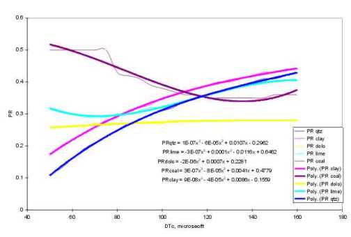
In the absence of good shear sonic data, Poison's Ratio can be estimated from the graph below, based on known or assumed lithology (courtesy Barree and Associates).
The
equations on this graph are: A high Poisson’s ratio indicates high stress level, which in turn indicates possible boundaries to a hydraulic fracture. Low Poisson’s ratio indicates weak zones which may not constrain the frac job, resulting in communication to undesired formations. Most shales constrain fractures but some may not do so. Two to three meters of rock with a Poisson's Ratio greater than 0.26 is the minimum needed to constrain a typical hydraulic fracture. Gas zones, where the sonic compressional data has not been corrected for gas, will show abnormally low Poisson's ratio. Poisson’s ratio is used to predict fracture pressure gradient in consolidated formations (Section 20.10).
For
rock with no porosity: Where:
If the rock is anisotropic, both Kb and Km can be calculated for the minimum and maximum stress directions by using DTSmin and DTSmax from a crossed dipole shear sonic log. Density is in gm/cc, travel time is in usec/ft, and Kb is in psi * 10^6 for English units. Density is in kg/m3, travel time is in usec/m, and Kb is in Giga-Pascals (10^9 Pa or GPa) for Metric units. If you like quicklook charts, here is one for Kb:
For
rock with porosity: For
rock with no porosity: This term is called rock compressibility and abbreviated Cr in some literature. If the rock is anisotropic, both Cb and Cm can be calculated for the minimum and maximum stress directions by using DTSmin and DTSmax from a crossed dipole shear sonic log. N and Cb predict sanding (sand production) in unconsolidated formations. When log analysis shows sanding may be a problem, sand control methods (injection of plastic or resin or gravel packing) can be initiated. Sanding is not a problem when N > 0.6*10^6 psi. in oil or gas zones. High water cuts increase the likelihood of sanding. This threshold corresponds to Cb of 0.75*10^-6 psi^-1. N/Cb > 0.8*10^12 psi^2 is a more sensitive cutoff than either N or Cb cutoffs. High N/Cb ratios indicate low chance for sanding. A good cement job is also needed to reduce sanding.
For
rock with porosity: For rock with no porosity, Kb = Km so ALPHA = 0. If
shear travel time is unavailable, this empirical relation may
be useful: where KS8 has the range 2 to 3, with KS8 = 3 most often used.
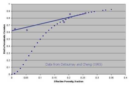
In
the absence of good shear sonic data, Biot's Constant can be estimated
from the graph above, based on known or assumed lithology (courtesy Barree and Associates). This graph suggests KS8 in the previous
equation is greater than 2.0. The empirical straight line fit to
the data is:
For
rock with porosity: If the rock is anisotropic, Y can be calculated for the minimum and maximum stress directions by using DTSmin and DTSmax from a crossed dipole shear sonic log when calculating N and P. Young's modulus calculated from log data is often called the dynamic Young's modulus, Ydyn. Young’s modulus is used in the fracture width (aperture) calculation in fracture design software. Here is the quicklook chart for Young’s modulus:
In the absence of good shear sonic data, Young's Modulus can be estimated from the graph below, based on known or assumed lithology (courtesy Barree and Associates). The ordinate on this graph is Young's Modulus divided by density (gm/cc), so multiply the Y axis value by density to obtain Y.
The equations on the above graph
are:
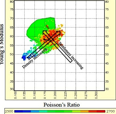
Where: Young's Modulus vs Poison's Ratio: Brittleness increases toward top left, density increases toward top right, porosity plus organic content and depth decrease toward bottom left. PR values less than 0.17 indicate gas or organic content or both. (image courtesy Canadian Discovery Ltd)
Glorioso offers a
direct brittleness indicator based solely on the lithologic
composition of the rock (SPE 153004, 2012). This paper was
specifically written for shale gas cases, which have naturally low
porosity, and this index may not be useful in more porous
rocks unless a porosity term is added to the denominator.
For rock with no
porosity, Kp = 0 and Kb = Km, and N = No, so:
The above calculations assume that fluid compressibilities are known from lab measurements of produced fluids. In recently drilled wells, this information is not always available. It would therefore be useful to predict fluid compressibility or fluid bulk modulus and use this result to predict the fluid type in the reservoir. A method using pore bulk modulus is more convenient, and is based on some empirical evidence for sandstones.
By setting
Kb = Km - 0.9 * N in equation 3, and solving for Kp: Kp is sometimes shown as Kf in the literature so be careful. Murphy (1991) provided equations for sandstone rocks (PHIe < 0.35) that predict Kb and N from porosity: 1: Kb = 38.18 * (1 - 3.39 * PHIe + 1.95 * PHIe^2) 2: N = 42.65 * (1 - 3.48 * PHIe + 2.19 * PHIe^2)
These
equations are for the water filled case and cannot be used as fluid
identification, but they may have other uses.
Unfortunately, the difference between dynamic (well log) values and static (lab) values on cores can be quite large, leading some people to dismiss the log data as wrong or useless. What makes this worse is that fracture design software has been calibrated to static (lab derived) values, so dynamic data has to be transformed to equivalent static numbers. Static values differ from dynamic values because wave propagation is a phenomenon of small strain with a large strain rate: rocks appear stiffer in response to an elastic wave, compared to a rock mechanics laboratory (triaxial) test, where larger strains are applied at lower strain rate. The weaker the rock, the larger the difference between elastic properties derived from acoustic measurements (dynamic) and those derived from triaxial measurements (static). This accounts for the marked difference between dynamic and static Young’s moduli. However, the difference between dynamic and static Poisson’s ratio is very small, and is generally not considered. There are further considerations. Since the tiny core plugs used for lab work have been de-stressed and re-stressed a number of times, there is some doubt that this cycle is truly reversible, so lab measurements may not represent in-situ conditions. The difference between static and dynamic values are larger for higher porosity, which suggests that some grain bonds are easily broken by coring and subsequent testing. It might be a wise move to calibrate fracture design software to dynamic data, since this data is more readily available, and may actually have fewer inherent measurement problems. Further, the effects of reservoir anisotropy cannot be simulated in the lab, so there is no reason to expect lab data to match in-situ log results. A possible solution to this dilemma is described in later Sections.
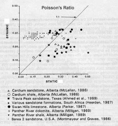
Doug Boyd (1991) presented a summary of published Poisson's Ratio data, shown at the right. As you can see, there is no direct relation between dynamic and static Poisson' ratio. Additional reasons for the mismatch might include dry rock measurements (as opposed to restored state), moisture variations in shaly samples, closing of fractures, pore shape changes, anisotropy (especially if core plugs are used instead of whole core), inconsistent (and often unknown) experimental methods, and experimental measurement error. Results of such a comparison made today might be less erratic if anisotropic effects were reduced by use of crossed dipole shear sonic data and appropriate core handling procedures. Calibration of local data seems possible, but there is no universal correction factor. When field measured closure stress is available from mini-fracs, a calibration of Poisson's Ratio is fairly easy in a homogenous reservoir, but probably impractical in many cases.
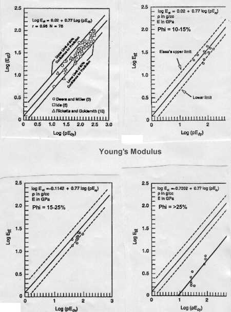
1: Yst = 10^(A + B * log(Ypsi)) Where: A and B are constants that depend on porosity as shown below:
This transform was based on high frequency dynamic lab data compared to static lab data. Low frequency log data was not used so this widely used transform may have no validity for log derived results. The
same paper quoted other data sets and compared their data to a
transform by Eissa. Note that these transforms invoke the rock
density to normalize the data. The equations are:
Lacy proposed a
correlation to obtain static Young's Modulus, Yst, from Ydyn. First
convert Ydyn to English units: NOTE: Results are in GPa. Divide by 6.894 to get psi * 10^6.
Barba's
correlation for Yst is:
|
|
||||||||||||||||||||||||||||||||||||||||||||||||||||||||||||||||||||||||||||||||||||||||||||||||||||||||||||||||||||||||||||||||
|
Page Views ---- Since 01 Jan 2015
Copyright 2023 by Accessible Petrophysics Ltd. CPH Logo, "CPH", "CPH Gold Member", "CPH Platinum Member", "Crain's Rules", "Meta/Log", "Computer-Ready-Math", "Petro/Fusion Scripts" are Trademarks of the Author |
|||||||||||||||||||||||||||||||||||||||||||||||||||||||||||||||||||||||||||||||||||||||||||||||||||||||||||||||||||||||||||||||||

|
||
| Site Navigation | ROCK PHYSICS CALCULATING MECHANICAL PROPERTIES | Quick Links |

 Errors
in Poisson's ratio strongly affect calculation of in-situ closure
stress.
Errors
in Poisson's ratio strongly affect calculation of in-situ closure
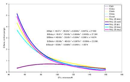
stress.  Young’s
modulus is also affected by differences between static and dynamic
values. A transform published by Morales and Marcinew in 1993
is shown in the graph on the left and formulated as:
Young’s
modulus is also affected by differences between static and dynamic
values. A transform published by Morales and Marcinew in 1993
is shown in the graph on the left and formulated as: