Productivity from Drill Stem Tests
To check the flow capacity (Kh) calculated from log analysis, it is sometimes helpful to calculate the flow capacity from an open hole drill stem test or a cased hole perforation or production test. Comparison can only be done for non-fractured and un-stimulated reservoirs because the open hole logs see the reservoir before fracturing or acidizing has taken place. If you believe that stimulation offers a constant increase in well productivity, then the log analysis permeability parameters can be adjusted to reflect this.

The Horner method is used for oil, water, or high pressure gas production. The Ramey method is used for low pressure gas wells. A spreadsheet called META/DST is available on the Downloads tab at www.spec2000.net  that makes the work relatively painless.

The mathematical solutions on this page were derived from Hugh W. Reid's DST Analysis course notes. Hugh presented his courses for many years in every oil capital on the planet. He specialized in finding by-passed pay, in spite of tests that were too short, or leaked, or which contained inaccurate pressure gauges. Unfortunately, that skill is not embedded in the math as it takes years of experience to recognize the knowledge hidden in poor quality data. To some degree, the Horner and Ramey Plot methods shown here have been replaced by pressure transient software that relies on curve fitting or curve matching models, but if you have older analog records of a valid test, Hugh's methods will work well as a first estimate of flow capacity.

Sadkt, Hugh passed away in March 2018 - his cheerful presence will be missed by many.
 

Horner Plot Method

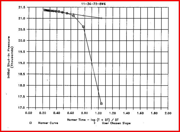
The Horner plot is a crossplot of buildup (or drawdown) pressure (Pi) on the Y axis versus a dimensionless time coefficient (HTi), usually called Horner Time, on a logarithmic X axis. A typical Horner plot is given below..

STEP 1: Calculate Horner time

 For Initial or Preflow portion of test:

 1: HTi = Log ((IFT + DTi) / DTi)

 For Final flow portion of test:

 2: HTi = Log (((IFT + FFT) + DTi) / DTi)

Where:  HTi = Horner time at point (unitless)

 DTi = Time since initial or final shut in for point (min)

 Pi = Initial or final flowing pressure (psi or KPa)

 IFT = Initial flowing time (min)

 FFT = Final flowing time (min)

Plot graph of Horner Time vs Shut-in Pressure as shown below.

STEP 2: Use data from graph to calculate slope of straight line portion of Horner plot:

 3: DSTslope = ABS (SIPend - SIPstart) / (HTend - HTstart)

Where: "start" represents start of straight line portion of Horner plot  "end" represents end of straight line portion of Horner plot

Calculate extrapolated shut in pressure:

 4: SIPextr = SIPend + DSTslope * HTend

STEP 3: Calculate actual DST flow rate

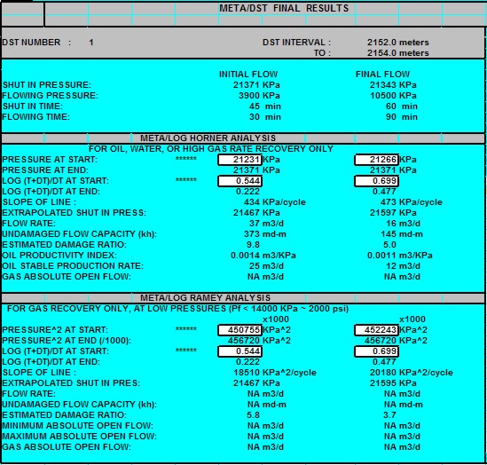
 5: Qoi = IFP / FFP * DSTrec / IFT * 1440

 6: Qgi = INITL DST gas rate

 7: Qof = (1 - IFP / FFP) * DSTrec / (IFT + FFT) * 1440

 8: Qgf = FINAL DST gas rate

STEP 4: Calculate flow capacity

 9: Khoil = KQ1 * Qo * 1/Bo * VISO / DSTslope

10. Khgas = KQ2 * Qg * Zg * VISG * KQ3 * (FT + KT2) / DSTslope /(SIPextr + IFP)

Where:  KQ1 = 162.6 for English units

 KQ1 = 2149 for Metric units

 KQ2 = 162.6 for English units

 KQ2 = 2.149 for Metric units

 KQ3 = 4.5 for English units

 KQ3 = 175.9 for Metric units

 KT2 = 460 'F for English units

 KT2 = 273 'C for Metric units

NOTE: This can be done for each buildup or drawdown period.  Qo is in bbl/day or m3/day; Qg is in mcf/day or m3/day. Pressure buildups on Repeat Formation Tester (RFT) can also be analyzed with this method.

STEP 5: Calculate productivity data

 11: Dratio = (SIPextr - IFP) / DSTslope / (log (IFT) + 2.65)

 12: Dratio = (SIPextr - FFP) / DSTslope / (log (IFT + FFT) + 2.65)

 13: PIo = KQ4 * Khoil / 1/Bo / VISO / (ln (10000) - 0.75 + 7 * (Dratio - 1))

Where:  KQ4 = 0.00708 for English units

 KQ4 = 53560 for Metric units

 14: AOFo = PIo * (SIPextr - IFP)

 15: AOFg = Khgas*(SIPextr+KP2)^2)/(KQ5*(FT+KT2)*Zg*VISG)/(ln(10000)-0.75+7*(Dratio-1))

Where:  KQ5 = 1424 for English units

 KQ5 = 1.309 for Metric units

 KP2 = 14.7 psi for English units

 KP2 = 101 KPa for Metric units

 KT2 = 460 'F for English units

 KT2 = 273 'C for Metric units

NOTE: AOFo is in bbl/day or m3/day; AOFg is in mcf/day or m3/day.

Ramey Plot Method

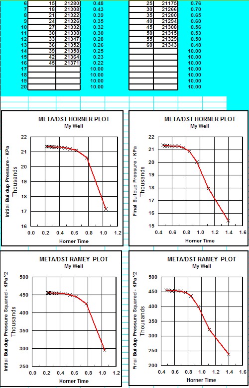
The Ramey plot is a crossplot of buildup (or drawdown) pressure squared (Pi^2) on the Y axis versus a dimensionless Horner Time, on a logarithmic X axis. The analysis arithmetic for SIP and Dratio are identical to that for the Horner method, except that pressure squared is substituted where ever pressure occurs in the equations. Also, the KHoil and AOFoil equations are not used. A typical Ramey plot is given below.

 1: Khgas = KQ6 * Qg * Zg * VISG * (FT + KT2) / DSTslope

Where:  KQ6 = 1637 for English units

 KQ6 = 1.508 for Metric units

 KT2 = 460 'F for English units

 KT2 = 273 'C for Metric units

 2: AOFmin = Qg * SIPextr / ((SIPextr ^ 2 - IFP ^ 2) ^ 0.5)

 3: AOFmax = Qg * SIPextr ^ 2 / (SIPextr ^ 2 - IFP ^ 2)

 4: AOFg = Khgas*((SIPextr+KP2)^2)/(KD5*(FT+KT1)*Zg*VISG)/(ln(10000)-0.75+7*(Dratio-1))

Where:  KD5 = 1424 for English units

 KD5 = 1.309 for Metric units

 KP2 = 14.7 psi for English units

 KP2 = 101 KPa for Metric units

 KT1 = 460 'F for English units

 KT1 = 273 'C for Metric units

NOTE: AOFg is in mcf/day or m3/day.
 

 
Horner Plot analysis of DST pressures
 

COMMENTS 

·      Use only for stabilized buildup.

·      Use to calibrate logs only if zone is not fractured, has not been stimulated, and exceeds 160 acres in size.

·      The Horner method is used for oil, water, or high pressure gas production.

·      The Ramey method is used for low pressure gas wells.

·      The flow capacity calculated from the equations shown above is for the damaged condition of the reservoir. The AOF result has the damage effect removed.

·      To compare Kh from logs with Kh from DST, the Kh from DST should be corrected for damage by the same factor as used in the AOF equation.

·      Results may not compare to log analysis for many reasons, such as insufficient build up time, reservoir boundaries, vertical barriers, fractures, and reservoir in-homogeneity. In addition, the log analysis flow capacity must be summed over the same interval as drained by the DST.
 

DST quality control is crucial. The Horner and Ramey methods only apply to valid tests which exhibit no boundary effects. DO NOT attempt Horner or Ramey analysis on an inappropriate DST curve.

META/LOG "DST" -- Pressure Transient Analysis by Horner Plot Method
This spreadsheet plots Pressure Buildup curves using "Quick Look" Horner and Ramey methods.

Download this spreadsheet:
SPR-20 META/LOG PRESSURE TRANSIENT CALCULATOR
  Calculate pressure buildup, and flow capacity from Horner and Ramey plots.

Sample output from "META/DST" spreadsheet showing input data, Horner plots and calculate
 flow capacity (KH) values.