Illustrative examples of crossplots, raw logs, answer plots, and tables of results, for example net pay summaries, are commonly included. Equations should be used only to explain a concept - the complete computer code is not required. Copies of all depth plots are usually delivered with the report as separate electronic images. Tables are also delivered separately as electronic spreadsheets.
A typical petrophysics report contains some or all of the following topivs: 1. Introduction or Executive Summary: this should include who the job was done for, the overall objective of the project, names and locations of wells and zones of interest, and a brief geological / mineralogical description of the zones of interest. 2. Data Available; describe log types and ages, core, XRD, petrography, sample descriptions, perforation and test intervals, production histories; comment on quality of each and especially what was missing that could have been useful. 3. Analysis Method; in words, explain the individual method used to calculate shale volume, porosity, lithology, water resistivity, water saturation, permeability, and net pay; describe how parameters were selected, and how well log analysis results match core and lab data; keep equations to a bare minimum. In unconventional reservoirs, describe what factors about the reservoir are unconventional and describe how additional parameters such as TOC weight fraction and kerogen volume were calculated. If mechanical properties were calculated, describe the log reconstruction method, list the basic properties that were derived, and the presence of any lab data that might be used for calibration. 4. Discussion of Results; may be omitted if covered in methodology; compare log analysis results to core and lab data, production history, etc, on a well by well basis. 5. Conclusions and Recommendations; discuss data quality, results quality compared to core, missing data, further lab work needed; come to a conclusion - the well (pool, project) is ...... 6. Disclaimer; you were not there, you didn't do it, and it's not your fault anyway. Your name is on the report, be proud of it. Log analysis reports hang around in well files for years. Don't leave a shoddy product that will come back to haunt you. Use clear, positive statements. Write as if talking out loud to an equal, but keep it organized and logical. Every sentence needs at least one noun and one verb. We all learned to do this in high school physics lab, so it's not really that hard. Keep it short and sweet - most petrophysical reports on small projects are less than five pages of text plus cover page and tables of results. A full field study may contain hundreds of pages from numerous authors, with geology, geophysics, engineering, and simulation sections, 100's of maps and graphs and well log displays. Keeping all this well organized and useful will take some skill and effort. Short reports don't need an executive summary but long reports definitely do. Long reports also need a table of contents, table of illustrations, and a clearly organized structure. "Requisite to a clear understanding of the interpretation of mud-gas data is consideration of the source of hydrocarbons as they occur in the drilling mud. To assist in this consideration, a simple drilling model is proposed which illustrates the impact of bit penetration through hydrocarbon accumulations. A series of cases is presented where variations in the configuration of the mud-gas data indicated specific differences in the response of the hydrocarbon bearing zone to bit penetration and subsequent rig operations. The model will show that the geometry of the gas kick recorded by the instrumentation and plotted with respect to time is directly related to significant characteristics of the hydrocarbon zone as well as the impact of concurrent drilling operations. It will become apparent that the configuration of the gas kick as recorded directly from the drilling mud is of greater interpretive significance than the magnitude of the gas kick. When instrument chart data recorded versus time is digitized and plotted in graph format versus depth, the magnitude of the gas kick may be faithfully reproduced but the configuration of the kick is usually lost. Thus it becomes obvious that basic and vital interpretation must derive from a detailed analysis of the instrument charts themselves and not solely from a plotted graph. The basic function of the plotted graph should be to collate, according to depth, pertinent data produced from various sources. This graph then provides a broader understanding of the hydrocarbon accumulation and a convenient means for future reference. To illustrate these concepts, a diagrammatic technique has been employed which graphically relates the gas detector response plotted versus time to the actual penetration of the rock by the drilling bit through the penetration rate curve plotted versus depth. This technique allows direct comparison of the geometry of the gas kick to actual rock penetration."
Scroll down to see four different, easy to read Petrophysical
Reports.
Petrophysical Analysis Report - Conventional
Reservoir
Introduction
Available
Data A Fm: T Fm: An analyzed core was available just below the main porous interval in the T Fm. Reported depths on this core appear to be 11 meters shallow (approx one pipe joint). A second, deeper core was not analyzed. No core was taken in the A Fm.
The top of the T Fm was tested through perforations and produced some wet gas. Eight separate intervals in the A Fm were tested through perforations, indicating wet gas in the lower 50 meters. No Rw data was provided, so water saturation values from log analysis are somewhat conjectural. No special core capillary pressure data is available to help calibrate water saturation.
Analysis Method
Porosity was determined by the sonic log corrected for shale. The density was also tried, but gave misleading results due to poor borehole condition.
Water saturation was derived with the Simandoux equation which corrects for the effects of shale. An Rw equivalent to 85000 ppm NaCl was used to achieve reasonable water saturations in the T Fm. A value approximating 45000 ppm was used in the A Fm. There are no obvious water zones, no RW data from offset wells, and no capillary pressure data to calibrate water saturation results.
A generic permeability curve using the Wyllie equation was generated but not presented on depth plots, as core permeability is much lower than the estimated values from this method.
Reasonable cutoffs were chosen from experience in tight sands and hydrocarbon summaries were printed. The zones that passed all cutoffs are flagged on the depth plots.
Depth plots at 1:1000 scale, brief summary listings, and this report were FAXed to Some One on 24 Month 2012. Hardcopy with plots at 1:500 scale were delivered by courier.
Results
Upper
T Fm: xxxx - xxxx mKB Phi = 0.093, Sw = 0.43, Net = 6.4 m This zone was perforated and tested gas.
Middle
T Fm: xxxx - xxxx mKB Phi = 0.121, Sw = 0.27, Net = 6.4 m This zone is not tested.
Lower
A Fm: xxx - xxx mKB Phi = 0.113, Sw = 0.51, Net = 50.4 m Eight zones within this interval were perforated and tested some gas. Additional intervals are untested and are flagged on the depth plots. Upper A Fm: xxx - xxx mKB Water saturation is speculative so no summations have been run. Numerous resistivity bumps indicate cleaner sands in thin intervals which might be gas bearing or they might contain fresher water, analogous to the Belly River in Alberta.
The lack of adequate density and neutron log data prevents the calculation of porosity corrected for heavy minerals. Since volcanic rock fragments can occur in large quantities in some sands, the porosity shown here could be several porosity units too low. The sonic log was calibrated to the core porosity in T Fm, but this core is in poor quality rock. This does not calibrate the higher porosities. No calibration was possible in A Fm.
Lack of a uranium corrected gamma ray log (CGR) hampers shale calculations. The overall high GR readings indicate either uranium salt precipitation (usually in fractures), feldspathic sands, or other radioactive rock fragments. It is impossible with this data set to separate these events from the shale content. Porosity calculations are suspect because of this.
Log character and borehole condition indicate a highly stressed, probably fractured, reservoir.
Results show many individual sands that probably contain gas. Any one of these could be leaking through poor cement to surface, or leaking and charging lower pressure water zones uphole.
A study should be undertaken to map water resistivity versus depth in the region, since no RW data was provided for this project.
In future wells, conventional and special core analysis to obtain capillary pressure and electrical properties should be contracted to help calibrate water saturation.
If possible, available core should be re-analyzed, described, and special core analysis properties obtained as soon as possible to allow recalibration of this log analysis.
INTRODUCTION
Final results of the
petrophysical analysis will be used to assist in assessment of
reservoir quality and to assist in stimulation design.
AVAILABLE DATA
No conventional, side-wall, or shale rock core analysis data were provided. Capillary pressure data was provided for three samples. Total organic carbon analysis and X-Ray diffraction mineralogy data was provided for one well.
ANALYSIS PROCEDURE Digital log data was provided by the client. These data were analyzed with a complex lithology petrophysical model, which accounts for the effects of heavy minerals and gas, using our proprietary META/LOG analysis script, running in the PowerLog software package.
TOC and XRD mass fraction lab measurements were converted to volume fractions based on the component densities. These were used to calibrate the kerogen correction to crossplot porosity and to calibrate clay and mineral volumes in the b-040 -I/094-O-05 well. The parameters and scale factors derived here were used in the other two wells.
Shale volume was calculated from the total gamma ray curve using a Clavier correction. Individual clean and shale lines were chosen for each zone in each well. Because of the effect of uranium on the total gamma ray curve, clean and shale lines were adjusted by comparison with the shale volume calculated from the density-neutron separation method. The final shale volume was calculated from the average of the two methods. Results match the clay volume fraction available from XRD data in well XXX.
Total organic carbon (TOC) was calculated using the Issler method with resistivity and density data, and calibrated to the lab data with scale and offset factors based on the available lab data in well XXX. The log derived TOC mass fraction matches the available lab data extremely well. The mass fraction curve was then converted to volume fraction for use in the porosity calculation.
Porosity was calculated from the shale corrected complex lithology density neutron crossplot model. The results from this model are relatively independent of mineralogy and compensated for gas effects. However, the effect of kerogen volume is included in this initial result, so the kerogen volume is subtracted to obtain the final effective porosity value.
There is no core porosity data to help calibrate this result. However, there is a nuclear magnetic log with effective porosity in d-34-K/094-O-05. This curve matches the calculated effective porosity curve in that well quite closely. The NMR effective porosity is unaffected by kerogen and is the best available check on the final effective porosity in this project.
The PE curve in XXX well was affected by barite weighted mud. It was reconstructed from multiple regression based on data in the other two wells.
The dominant lithology is described as quartz (with clay), some calcite (increasing somewhat with depth), and minor pyrite. This would need a three mineral log analysis model since the effect of pyrite on the lithology calculation can be quite significant. Because of gas effect, lithology models that use the density or neutron log data cannot be used, leaving only a two-mineral model based on PE available.
To account for pyrite, pyrite volume was derived from a multiple regression using all available lithology indicating logs, calibrated to the XRD pyrite volume. This curve was then used to remove the effect of pyrite from the PE curve, allowing it to be used in a 2-mineral model.
Lithology was then calculated with a 2-mineral model using the pyrite corrected PE data, with a mineral mixture chosen as quartz and calcite. The final result is a three mineral model with quartz, calcite, and pyrite (and clay) that matches the XRD data quite well. All TOC and XRD data points are plotted on the log analysis depth plots for comparison.
The Simandoux equation was used for water saturation calculations. This model reverts to the Archie equation in the clean zones.
Water resistivity was set at 0.060 ohm-m at 25C for all zones. Electrical properties were set at A = 1.00, M = N = 1.65. Formation temperature gradient was set at 3.13C / 100 m with a surface temperature of 10C. This gives a formation temperature of 86C at 2430 meters.
No lab measured electrical properties were available; those used are based on prior experience in tight sands.
A permeability index was generated from a standard relationship; the equation is Perm = 10^(20.0 * PHIe – 2.0). There is no core data for calibrating this value so it should be treated as a qualitative guide. The permeability derived from the Coates equation was provided for the NMR log in d-34-K. It has been plotted on the depth plot for comparison to our calculated results. These permeabilities do not include that from natural fractures or stimulation.
We were requested to calculate the acoustic anisotropic coefficient of the interval, based on differences between the X and Y axis crossed-dipole sonic log data. Even on an expanded scale log, there was no significant difference between the two log curves. We conclude that the acoustic anisotropic coefficient (Kani) is zero.
Using the complete petrophysical analysis results described above, reconstructed log curves were generated. This step removes bad hole and gas effects from the logs so that accurate water-filled rock mechanical properties can be calculated. This process is also used to create missing log curves where needed.
Calculated mechanical properties include Biot’s constant, bulk, shear, and Young’s moduli, and Poisson’s Ratio. A brittleness coefficient (Lame’s constant, Lambda) was also calculated. These results are displayed, along with the lithology track, on a separate depth plot.
These results are not calibrated as there is no lab data available. However, all results are within normal limits for water-filled rocks of this type and are suitable for use in stimulation design programs.
Use of the raw log curves instead of the reconstructed logs should be strongly discouraged because the gas effects are quite large and will lead to calculation of erroneous stimulation parameters.
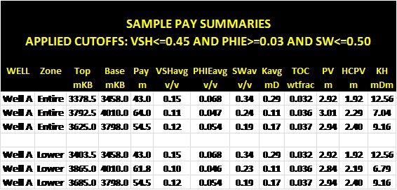
RESULTS
NET PAY SUMMARIES
All data in the above tables are based on measured log depths.
Free gas in place can be calculated from these data using appropriate gas volume factor, temperature, pressure, and area.
The Trican report provided by the client indicated that adsorbed gas volume would be small. In any case, adsorbed gas volume cannot be calculated from the log analysis as there is no gas content (Gc) versus total organic carbon (TOC) relationship available in the data set provided.
Results of the log analysis of the wells are contained in the depth plots, LAS files, and net pay spreadsheet delivered with this report. All depth plots are measured depth displays.
CONCLUSIONS
The permeability index provided in our work should only be used qualitatively.
Mechanical rock properties calculated from these results are believed to be reliable and can be used as input to stimulation design software.
Results match available TOC and XRD data. However, there is no useable porosity or permeability control data from conventional or sidewall cores. Confidence in this analysis could be markedly improved if a cored well was added to the well complement.
Formation tops, formation names, and perforation intervals were provided by the client, and were used on our answer and raw data plots for zone identification purposes only. We express no opinion on the correctness of the name designations or associated depths.
This is not a reserves or resource appraisal report.
Respectfully submitted
E. R. (Ross) Crain, P.Eng.
Disclaimer
All interpretations expressed in this report, and contained in any
attachments thereto, are opinions based on inferences from
geophysical well logs and/or laboratory measurements provided by the
client.
SAMPLE
REPORT #3 Introduction We were requested
to review the log, core, and production test information provided by
Company B on seven wells in the
Available Data Raw data depth
plots of the well logs for the seven wells were provided. These were
re-plots from a log analysis software package and not the original logs.
Typical log suite included gamma ray, SP, caliper, deep and shallow
resistivity, density, neutron, sonic, and PEF (in newer wells). No
spectral gamma ray data was recorded. This would have been very useful in
accounting for the feldspar and other possibly radioactive rock fragments
in the sands.
Discussion of Petrophysical Computations The petrophysical
computation and display of results for five of the seven wells (N-3, 6,
7, 5, and 4) is excellent, with one major problem, discussed below.
Recommendations 1. Assemble all core
data, classify as to source (sidewall, whole core, plugs),
and review for consistency and usefulness. Re-plot core
porosity vs core permeability. List and compare thin section
visual porosity to core porosity.
Research
Petrophysics Report Introduction The interval of interest is from sea floor to the top of Chalk or top of Zechstein evaporites if Chalk is not present. The main pay zones are the Montrose sands lying above the Chalk. The
objective of this project is to evaluate the efficacy
of the standard overpressure indicator method based
on sonic log trend line analysis. The approach
is commonly known as the Eaton method, but similar
discussions have been published many years earlier. Formation pressure data for the Montrose were provided for six wells. A
report from the client was provided, which contained
discussion and results of their analysis using
the Eaton method on a number of wells. Shale volume was determined from the gamma ray log. Porosity was determined by the sonic log corrected for shale. The density neutron crossplot porosity was also calculated where possible. No water saturation calculation was made. The equations used were: Neutron
porosity Density
Porosity Sonic
Porosity Shale
Volume Effective
Porosity GRcl and GRsh were chosen uniquely for each well. These results were used to determine shale beds suitable for analysis of overpressure by the Eaton method. Data below the zone of interest (Montrose) was deleted from the working files after this analysis step. The calculation steps for the Eaton method are listed below: Actual
shale travel time Normal
shale travel time compaction trend line Difference
between actual and normal sonic values Overburden
pressure Shale
Pore Pressure as a gradient Shale
pore pressure as head of water Shale
pore pressure as a pressure RFT
pressure from lookup table RFT
pressure as a head of water DTnorm is the sonic trend line chosen in a shallow shale zone to represent the normal compaction trend. The position and slope of this line is very subjective. The line finally chosen is very similar to the line used by the client. My first pick fits the sonic log better but gave less overpressure than my final pick. There is, in fact, very little valid sonic data in the shallow sequence to which a line can be fitted. Depth plots of both my initial and final lines, along with the sonic log curves for 7 wells, are provided under separate cover. The final line was picked to account for actual mud weights used to maintain the holes and to approximate actual Montrose reservoir pressures at the top of the gas/oil column. SOV is the overburden stress. This equation varies from place to place. It was supplied by the client and is assumed to be suitable for this region of the North Sea. SPP is the shale pore pressure from the Eaton equation. It is converted to meters of head of water (SPP-M) and to pressure in KPa (PRESsh). For comparison, the RFT pressures for any depth were found in a lookup table (psi) and converted to head in meters and pressure in KPa. Depth
plots at 1:10,000 scale were made of all these
results plus the raw log data. A lithology track
was created from the Vsh curve and a depth function
related to the formation name. Thus sandstone,
limestone (chalk), anhydrite, and salt were shown
where appropriate. The final compaction trend line was chosen as a compromise. The initial choice generated very little overpressure, yet mud weight data supplied by the client suggested higher pressure results were needed to account for the mud weights actually used. The final choice was arrived at after several iterations. The final trend gives shale overpressure values close to actual mud weight gradients and close to actual formation pressures at the top of the Montrose structure. Matching
the actual Montrose pressure is not a requirement
of the method. A normally pressured shale is sufficient
to act as a seal, even for the relatively high
buoyancy caused by the large oil and gas column.
It should be noted that none of the Montrose data
shows significant overpressure in the reservoir.
The pressures are close to those expected for the
hydrocarbon buoyancy. The effect of a gas phase in porosity within the silt component of the shale cannot be accounted for, even if it were known to be present. Invasion by drilling fluid removes most of the gas from the region seen by the sonic log, so the effect should be very small. A well log model study could be undertaken to assess the magnitude of gas effect. Gas leaking through fractures would probably not influence this method. If the other unknowns described in the previous paragraph could be calibrated, it is unlikely that gas in the silt would pose additional problems, but the model study suggested above would quantify this. It should be noted that the seismic signal may be influenced by gas in porosity in the silty shales or in fractures. Seismic studies for detection of overpressure may be compromised by this effect, while the sonic log is not. The
validity of the Eaton method for calculation of
shale pore pressure has not been proven, since
there are no actual pressure data points within
the shale interval that can be used for calibration. Results should not be used as a quantitative measure of the amount of overpressure. Further work is required from this specific area to validate the overburden stress (SOV) formula, on which the Eaton method depends. Pressures must be acquired from stray sands within the overpressured shales to calibrate the terms in the Eaton equation for SPP and to validate the normal compaction curve (DTnorm) for use in this specific area.. There is no reason to believe that the parameters in these equations are universal constants and they need confirmation from this area to be used reliably in this area.
E.
R. (Ross) Crain, P.Eng. |
|
||
|
Page Views ---- Since 01 Jan 2015
Copyright 2023 by Accessible Petrophysics Ltd. CPH Logo, "CPH", "CPH Gold Member", "CPH Platinum Member", "Crain's Rules", "Meta/Log", "Computer-Ready-Math", "Petro/Fusion Scripts" are Trademarks of the Author |
|||

|
||
| Site Navigation | MANAGEMENT WRITING PETROPHYSICAL ANALYSIS REPORTS | Quick Links |

 Tables
of results and graphs are usually
copied to the text document. These should be embedded near the
appropriate text, if possible. Large tables may appear at the end of
the report.
Tables
of results and graphs are usually
copied to the text document. These should be embedded near the
appropriate text, if possible. Large tables may appear at the end of
the report.