
|
Although I learned all this in University 50+ years ago, I can no longer recite any of it from memory. Therefore, the following is from Wikipedia http://en.wikipedia.org/wiki/Maxwell's_laws , with a little editing. If you don't have strong calculus skills, most of this material will be meaningless. Have fun!
|
||||||||||||||||||||||||||||||||||||||||||||||||||||||||||||||||||||||||||||||||||||||||||||||||||||||||||||||||||||||||||||||||||||||||||||||||||||
| Symbol | Meaning (first term is the most common) | SI Unit of Measure |
|---|---|---|
|
|
the divergence operator | per meter (factor contributed by applying either operator) |
|
|
the curl operator | |
|
|
partial derivative with respect to time | per second (factor contributed by applying the operator) |
|
|
electric field |
volt per
meter or, equivalently, newton per coulomb |
|
|
magnetic field also called the magnetic induction also called the magnetic field density also called the magnetic flux density |
tesla, or equivalently, weber per square meter volt•second per square meter |
|
|
electric displacement field |
coulombs per
square meter or,
equivalently, newton per volt-meter |
|
|
magnetizing field also called auxiliary magnetic field also called magnetic field intensity also called magnetic field |
ampere per meter |
|
|
permittivity of
free space, officially
the
electric constant, a universal constant |
farads per meter |
|
|
magnetic
permeability of
free space, officially
the
magnetic constant, a universal constant |
henries per meter, or newtons per ampere squared |
|
|
free charge density (not including bound charge) | coulomb per cubic meter |
|
|
total charge density (including both free and bound charge) | coulomb per cubic meter |
|
|
the flux of the electric field over any closed gaussian surface S | joule-meter per coulomb |
|
|
net unbalanced
free
electric charge enclosed
by the Gaussian surface S (not including bound charge) |
coulombs |
|
|
net unbalanced
electric charge enclosed
by the Gaussian surface S (including both free and bound charge) |
coulombs |
|
|
the flux of the magnetic field over any closed surface S | tesla meter-squared or weber |
|
|
line integral of the
electric field along the
boundary ∂S (therefore necessarily a closed curve) of the surface S |
joule per coulomb |
|
|
magnetic flux over any surface S (not necessarily closed) | weber |
|
|
free current density (not including bound current) | ampere per square meter |
|
|
total current density (including both free and bound current) | ampere per square meter |
|
|
line integral of the
magnetic field over the closed boundary ∂S of the surface S |
tesla-meter |
|
|
net
free
electrical current
passing through the surface S (not including bound current) |
amperes |
|
|
net
electrical current
passing through the surface S (including both free and bound current) |
amperes |
|
|
electric flux through any surface S, not necessarily closed | joule-meter per coulomb |
|
|
flux of electric displacement field through any surface S, not necessarily closed | coulombs |
|
|
differential vector
element of surface area A,
with
infinitesimally small magnitude and direction normal to surface S |
square meters |
|
|
differential vector element of path length tangential to contour | meters |
![]() MODERN VERSIONS OF MAXWELL'S
LAWS
MODERN VERSIONS OF MAXWELL'S
LAWS
Two equivalent, general formulations
of Maxwell's equations follow. The
first separates
free charge and
free current from
bound charge and
bound current. This separation
is useful for calculations involving
dielectric and/or
magnetized materials. The second
formulation treats all charge
equally, combining free and bound
charge into total charge (and
likewise with current). Of course,
such an approach applies where no
dielectric or magnetic material is
present, and therefore no bound
charge or current, but it also is a
more fundamental or microscopic
point of view.
 Table 1:
Formulation in terms of free
charge and current
Table 1:
Formulation in terms of free
charge and current
| Name | Differential form | Integral form |
|---|---|---|
| Gauss's law: |
|
|
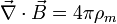
| Gauss's law for magnetism: |
|
|
|
Maxwell-Faraday equation (Faraday's law of induction): |
|
|
|
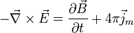
Ampère's Circuital Law (with Maxwell's correction): |
|
|
Table 2:
Formulation in terms of total
charge and current
| Name | Differential form | Integral form |
|---|---|---|
| Gauss's law: |
|
|
| Gauss's law for magnetism: |
|
|
|
Maxwell-Faraday equation (Faraday's law of induction): |
|
|
|
Ampère's Circuital Law (with Maxwell's correction): |
|
|
Maxwell's equations are generally applied to macroscopic averages of the fields, which vary wildly on a microscopic scale in the vicinity of individual atoms (where they undergo quantum mechanical effects as well). It is only in this averaged sense that one can define quantities such as the magnetic permittivity and magnetic permeability of a material. At the microscopic level, Maxwell's equations, ignoring quantum effects, describe fields, charges and currents in free space — but at this level of detail one must include all charges, even those at an atomic level, generally an intractable problem.
![]() SPECIAL CASES
SPECIAL CASES
Bound
charge, and proof that formulations
are equivalent
If an electric field is applied to a dielectric material, each of the molecules responds by forming a microscopic dipole -- its atomic nucleus will move a tiny distance in the direction of the field, while its electrons will move a tiny distance in the opposite direction. This is called polarization of the material. The distribution of charge that results from these tiny movements turn out to be identical to having a layer of positive charge on one side of the material, and a layer of negative charge on the other side -- a macroscopic separation of charge, even though all of the charges involved are "bound" to a single molecule. This is called bound charge. Likewise, in a magnetized material, there is effectively a "bound current" circulating around the material, despite the fact that no individual charge is traveling a distance larger than a single molecule. The relation between polarization, magnetization, bound charge, and bound current is as follows:
where P and M are polarization and magnetization, and ρb and Jb are bound charge and current, respectively. Plugging in these relations, it can be easily demonstrated that the two formulations of Maxwell's equations given above are precisely equivalent.
Constitutive Relations
In
order to apply Maxwell's equations
(the formulation in terms of free
charge and current, and D and H), it
is necessary to specify the
relations between D and E, and H and
B. These are called
constitutive relations, and
correspond physically to specifying
the response of bound charge and
current to the field, or
equivalently, how much
polarization and
magnetization a material
acquires in the presence of
electromagnetic fields.
Case
without magnetic or dielectric
materials
In the absence
of magnetic or
dielectric materials, the relations
are simple:
where ε0 and μ0 are two universal constants, called the permittivity of free space and permeability of free space, respectively.
Case of
linear materials
In
a "linear",
isotropic, nondispersive, uniform material,
the relations are also
straightforward:
where ε and μ are constants (which depend on the material), called the permittivity and permeability, respectively, of the material.
General
case
For real-world materials, the
constitutive relations are not
simple proportionalities, except
approximately. The relations can
usually still be written:
but ε and μ are not, in general, simple constants, but rather functions. For example, ε and μ can depend upon:
-
The strength of the fields
(the case of
nonlinearity, which
occurs when ε and μ are
functions of E and B; see, for
example,
Kerr and
Pockels effects),
-
The
direction of the fields (the
case of
anisotropy,
birefringence, or
dichroism; which occurs
when ε and μ are second-rank
tensors),
-
The
frequency with which the fields
vary (the case of
dispersion, which occurs
when ε and μ are functions of
frequency; see, for example,
Kramers–Kronig relations),
-
The
position inside the material
(the case of a nonuniform
material, which occurs when
ε and μ vary from point to point
within the material; for example
in a
domained structure,
heterostructure or a
liquid crystal),
- The history of the fields (the case of hysteresis, which occurs when ε and μ are functions of both present and past values of the fields).
Equations
in terms of E and B
for linear materials
Substituting in
the constitutive relations above,
Maxwell's equations in a linear
material (differential form only)
are:
These are formally identical to the general formulation in terms of E and B (given above), except that the permittivity of free space was replaced with the permittivity of the material (THIS CHAPTER displacement field, electric susceptibility and polarization density), the permeability of free space was replaced with the permeability of the material, and only free charges and currents are included (instead of all charges and currents).
Maxwell's
equations in vacuum
Starting with the equations
appropriate in the case without
dielectric or magnetic materials,
and assuming that there is no
current or electric charge present
in the vacuum, we obtain the Maxwell
equations in
free space:
These equations have a solution in terms of traveling sinusoidal plane waves, with the electric and magnetic field directions orthogonal to one another and the direction of travel, and with the two fields in phase, traveling at the speed.
The traveling wave solution is found by substitution of one of the curl equations into the time derivative of the other, producing:
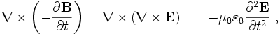
which reduces to the electromagnetic wave equation due to an identity in vector calculus. The equation is satisfied in one dimension, for example, by a solution of the form E = E( x − c0t ), that is, by a solution that is unchanged when t advances to t + Δt at a position x that advances to x + c0 Δt.
Maxwell discovered that this quantity c0 is the speed of light in vacuum, and thus that light is a form of electromagnetic radiation. The current SI values for the speed of light, the electric and the magnetic constant are summarized in the following table.
| Symbol | Name | Numerical Value | SI Unit of Measure | Type |
|---|---|---|---|---|
|
|
Speed of light in vacuum | 299 792.458 | meters per second | defined |
|
|
Electric constant |
8. 854 187 817 x 10^-12 |
Farads per meter |
derived
|
|
|
Magnetic constant | 1.2566 x 10^-6 | Henrys per meter | defined |
Nondimensionalization and
unobservability of the speed of
light
Because c0 and μ0
have defined values (they are
properties of the ideal reference
state of
free space), they are not
subject to alteration due to
experimental observation. For
example, if length is measured in
units λ and time in units τ, the
distance x in units of λ
becomes x = λ ζ and the time
t becomes t = τ η,
where ζ is the number of length
units in x and η is the
number of time units in t.
The above curl equation for
the traveling wave becomes:
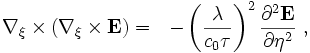
and because the SI units are related by λ = c0τ this equation does not depend any longer on the speed of light. Experiment could in principle, however, alter the standard meter, for example, as a result of greater
measurement accuracy.
With
magnetic monopoles
Maxwell's equations of
electromagnetism relate the electric
and magnetic fields to the motions
of electric charges. The standard
form of the equations provide for an
electric charge, but posit no
magnetic charge. Except for
this, the equations are symmetric
under interchange of electric and
magnetic field. In fact, symmetric
equations can be written when all
charges are zero, and this is how
the
wave equation is derived .
Fully symmetric equations can also be written if one allows for the possibility of "magnetic charges" analogous to electric charges. With the inclusion of a variable for these magnetic charges, there will also be "magnetic current" variable in the equations. The extended Maxwell's equations, simplified by nondimensionalization, are as follows:
-
Name Without Magnetic Monopoles With Magnetic Monopoles (hypothetical) Gauss's law: 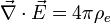

Gauss' law for magnetism: 
Maxwell-Faraday equation
(Faraday's law of induction):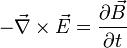
Ampère's law
(with Maxwell's extension):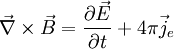

If
magnetic charges do not exist, or if
they exist but where they are not
present in a region, then the new
variables are zero, and the
symmetric equations reduce to the
conventional equations of
electromagnetism such as
![]() .
Classically, the question is "Why
does the magnetic charge always seem
to be zero?"
.
Classically, the question is "Why
does the magnetic charge always seem
to be zero?"
Materials
and dynamics
The fields in Maxwell's equations
are generated by charges and
currents. Conversely, the charges
and currents are affected by the
fields through the
Lorentz force equation:
where q is the charge on the particle and v is the particle velocity. (It also should be remembered that the Lorentz force is not the only force exerted upon charged bodies, which also may be subject to gravitational, nuclear, etc. forces.) Therefore, in both classical and quantum physics, the precise dynamics of a system form a set of coupled differential equations, which are almost always too complicated to be solved exactly, even at the level of statistical mechanics. This remark applies to not only the dynamics of free charges and currents (which enter Maxwell's equations directly), but also the dynamics of bound charges and currents, which enter Maxwell's equations through the constitutive equations, as described next.
Commonly, real materials are approximated as "continuum" media with bulk properties such as the refractive index, permittivity, permeability, conductivity, and/or various susceptibilities. These lead to the macroscopic Maxwell's equations, which are written (as given above) in terms of free charge/current densities and D, H, E, and B ( rather than E and B alone ) along with the constitutive equations relating these fields. For example, although a real material consists of atoms whose electronic charge densities can be individually polarized by an applied field, for most purposes behavior at the atomic scale is not relevant and the material is approximated by an overall polarization density related to the applied field by an electric susceptibility.
Continuum approximations of atomic-scale inhomogeneities cannot be determined from Maxwell's equations alone. but require some type of quantum mechanical analysis such as quantum field theory as applied to condensed matter physics. See, for example, density functional theory, Green–Kubo relations and Green's function (many-body theory). Various approximate transport equations have evolved, for example, the Boltzmann equation or the Fokker–Planck equation or the Navier-Stokes equations. Some examples where these equations are applied are magnetohydrodynamics, fluid dynamics, electrohydrodynamics, superconductivity, plasma modeling. An entire physical apparatus for dealing with these matters has developed. A different set of homogenization methods (evolving from a tradition in treating materials such as conglomerates and laminates) are based upon approximation of an inhomogeneous material by a homogeneous effective medium (valid for excitations with wavelengths much larger than the scale of the inhomogeneity).
Real world
issues
Theoretical results have their
place, but often require fitting to
experiment. Continuum-approximation
properties of many real materials
rely upon measurement, for example,
ellipsometry measurements.
In practice, some materials properties have a negligible impact in particular circumstances, permitting neglect of small effects. For example: optical nonlinearities can be neglected for low field strengths; material dispersion is unimportant where frequency is limited to a narrow bandwidth; material absorption can be neglected for wavelengths where a material is transparent; and metals with finite conductivity often are approximated at microwave or longer wavelengths as perfect metals with infinite conductivity (forming hard barriers with zero skin depth of field penetration).
And, of course, some situations demand that Maxwell's equations and the Lorentz force be combined with other forces that are not electromagnetic. An obvious example is gravity. A more subtle example, which applies where electrical forces are weakened due to charge balance in a solid or a molecule, is the Casimir force from quantum electrodynamics.
The connection of Maxwell's equations to the rest of the physical world is via the fundamental sources of charges and currents and the forces on them, and also by the properties of physical materials.
![]() Boundary
conditions
Boundary
conditions
Although Maxwell's equations apply
throughout space and time, practical
problems are finite and solutions to
Maxwell's equations inside the
solution region are joined to the
remainder of the universe through
boundary conditions
and started in time
using
initial conditions.
In some cases, like
waveguides or cavity
resonators, the solution region
is largely isolated from the
universe, for example, by metallic
walls, and boundary conditions at
the walls define the fields with
influence of the outside world
confined to the input/output ends of
the structure.
In other cases, the universe at
large sometimes is approximated by
an
artificial absorbing boundary,
or, for example for radiating
antennas or
communication satellites, these
boundary conditions can take the
form of asymptotic limits
imposed upon the solution.
In addition, for example in an
optical fiber or
thin-film optics, the solution
region often is broken up into
subregions with their own simplified
properties, and the solutions in
each subregion must be joined to
each other across the subregion
interfaces using boundary
conditions.
Following are some links of a
general nature concerning boundary
value problems:
Examples of boundary value problems,
Sturm-Liouville theory,
Dirichlet boundary condition,
Neumann boundary condition,
mixed boundary condition,
Cauchy boundary condition,
Sommerfeld radiation condition.
Needless to say, one must choose the
boundary conditions appropriate to
the problem being solved.
![]() THE HEAVISIDE
VERSIONS
THE HEAVISIDE
VERSIONS
Gauss's law
describes the relation between the
electric field and the distribution
of electric charge, as follows:
The formulation of
Table 1 is assumed; that is, ρf
is the "free" electric charge
density (in units of
C/m³),
not including
bound charge from the
polarization of a material, and
![]() is the
electric displacement field (in
units of C/m²). For stationary
charges in vacuum, the force exerted
upon one point charge by another as
found from Gauss's law is
Coulomb's law.
is the
electric displacement field (in
units of C/m²). For stationary
charges in vacuum, the force exerted
upon one point charge by another as
found from Gauss's law is
Coulomb's law.
The equivalent integral form (by the divergence theorem) of Gauss' law is:
where:
- S is any fixed, closed surface,
-
The
integral is a
surface integral, i.e.
 is a
vector whose magnitude is
the area of a differential
square on the closed surface A,
and whose direction is an
outward-facing
normal vector, and
is a
vector whose magnitude is
the area of a differential
square on the closed surface A,
and whose direction is an
outward-facing
normal vector, and
- Qenclosed is the free charge enclosed within the surface S. (If the surface itself is charged, that gives an extra contribution weighted by a factor 1/2.)
In a linear, isotropic, homogeneous material, with instantaneous response to field changes, D is directly related to the electric field E via a material-dependent constant called the permittivity, ε:
-
 .
.
The material permittivity ε can also be written as ε0 εr where εr is the material's relative permittivity or its dielectric constant. No material (except free space) is precisely linear and isotropic, but many materials are approximately so. The permittivity of free space, or electric constant, is denoted as ε0 (approximately 8.854 pF/m), and appears in:
where, again, E is the electric field (in units of V/m), ρt is the total charge density (including bound charges). The formulation of Table 2 is assumed.
Some insight into Gauss' law is found using the Maxwell-Faraday equation:
which shows the solenoidal portion of E is determined by the time variation of the magnetic field. Thus, in electrostatics (that is, when the system is unchanging in time), by Helmholtz decomposition the E-field can be expressed in terms of a scalar field as:
Time independence not only allows E to be expressed as a gradient, but also removes any time-delay in material response (ε independent of time), so the equation determining the electrostatic potential ɸ (r ) is:
which is Poisson's equation in the case where ε is independent of position (that is, when the material is homogeneous). The formulation of Table 1 is assumed. That is, the bound charge is subsumed under the permittivity, and only the free charge is explicit on the right side of the equation.
Gauss's law for magnetism states that the divergence of the magnetic field is always zero (in other words, the magnetic field is a solenoidal vector field):
where
![]() is the
magnetic B-field (in units of
tesla, denoted "T"), also called
"magnetic flux density", "magnetic
induction", or simply "magnetic
field". It is interpreted as saying
there is no "magnetic" charge that
is the analog of the electric
charge, and often this equation is
referred to as "the absence of
magnetic monopoles". Differently
put, the basic entity for magnetism
is the
magnetic dipole, which
orients itself in a magnetic field.
is the
magnetic B-field (in units of
tesla, denoted "T"), also called
"magnetic flux density", "magnetic
induction", or simply "magnetic
field". It is interpreted as saying
there is no "magnetic" charge that
is the analog of the electric
charge, and often this equation is
referred to as "the absence of
magnetic monopoles". Differently
put, the basic entity for magnetism
is the
magnetic dipole, which
orients itself in a magnetic field.
By the divergence theorem, the above divergence equation has an equivalent integral form:
where
![]() is an infinitesimal vector
corresponding to the area of a
differential square on the surface
S with an outward facing
surface normal defining its
direction.
is an infinitesimal vector
corresponding to the area of a
differential square on the surface
S with an outward facing
surface normal defining its
direction.
Like the electric field's integral form, this equation works only if the integral is done over a closed surface.
This equation is related to the magnetic field's structure because it states that given any volume element, the net magnitude of the vector components that point outward from the surface must be equal to the net magnitude of the vector components that point inward. Structurally, this means that the magnetic field lines must be closed loops. Another way of putting it is that the field lines cannot originate from somewhere; attempting to follow the lines backwards to their source or forward to their terminus ultimately leads back to the starting position. Hence, the above reference to this law as saying there are no magnetic monopoles.
The Maxwell-Faraday equation states:
This equation is usually referred to as "Faraday's law of induction", but in fact it is only a restricted form of Faraday's law; for example, it doesn't apply to situations involving motionally induced EMF.
Ampère's circuital law describes the source of the magnetic field,
where
![]() is the
magnetic field strength (in
units of
A/m),
related to the magnetic flux density
is the
magnetic field strength (in
units of
A/m),
related to the magnetic flux density
![]() by a constant called the
permeability, μ (
by a constant called the
permeability, μ (![]() ),
and
J
is the current density, defined by:
),
and
J
is the current density, defined by:
![]() where
where
![]()
![]() is a vector field called the drift
velocity that describes the
velocities of the charge carriers
which have a density described by
the scalar function ρq.
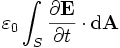
The second term on the right hand
side of
Ampère's Circuital Law is known
as the
displacement current.
is a vector field called the drift
velocity that describes the
velocities of the charge carriers
which have a density described by
the scalar function ρq.
The second term on the right hand
side of
Ampère's Circuital Law is known
as the
displacement current.
It was Maxwell who added the displacement current term to Ampère's Circuital Law at equation (112) in his 1861 paper On Physical Lines of Force.
Maxwell used the displacement current in conjunction with the original eight equations in his 1865 paper A Dynamical Theory of the Electromagnetic Field to derive a wave equation that has the velocity of light. Most modern textbooks derive this electromagnetic wave equation using the 'Heaviside Four'.
In free space, the permeability μ is the magnetic constant, μ0, which is defined to be exactly 4π×10-7 Wb/A•m. Also, the permittivity becomes the electric constant ε0, also a defined quantity. Thus, in free space, the equation becomes:
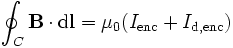
Using Stokes theorem the equivalent integral form can be found:
C is the edge of the open
surface A (any surface with
the curve C as its edge will
do), and Iencircled
is the current encircled by the
curve C (the current through
any surface is defined by the
equation:
![]() ).
Sometimes this integral form of
Ampere-Maxwell Law is written as:
).
Sometimes this integral form of
Ampere-Maxwell Law is written as:
-
 because the term
is displacement current. The displacement current concept was Maxwell's greatest innovation in electromagnetic theory. It implies that a magnetic field appears during the charge or discharge of a capacitor. If the electric flux density does not vary rapidly, the second term on the right hand side (the displacement flux) is negligible, and the equation reduces to Ampere's law.
MAXWELL'S EQUATIONS
IN CGS UNITS
The above equations are given in the
International System of Units,
or
SI for short. In a related unit
system, called cgs (short for
centimeter-gram-second), the
equations take the following form:
Where c is the speed of light in a vacuum. For the electromagnetic field in a vacuum, the equations become:
In this system of units the relation between magnetic induction, magnetic field and total magnetization take the form:
With the linear approximation:
χm for vacuum is zero and therefore:
and in the ferro or ferri magnetic materials where χm is much bigger than 1:
The force exerted upon a charged particle by the electric field and magnetic field is given by the Lorentz force equation:
where
![]() is the charge on the particle and
is the charge on the particle and
![]() is the particle velocity. This is
slightly different from the
SI-unit
is the particle velocity. This is
slightly different from the
SI-unit
expression above. For
example, here the magnetic field
![]() has the same units as the electric
field
has the same units as the electric
field
![]() .
.
Maxwell's
equations and special relativity
Maxwell's equations have a close
relation to
special relativity: Not only
were Maxwell's equations a crucial
part of the historical development
of special relativity, but also,
special relativity has motivated a
compact mathematical formulation
Maxwell's equations, in terms of
covariant tensors.
![]() MAXWELL'S ORIGINAL
EQUATIONS
MAXWELL'S ORIGINAL
EQUATIONS
The eight original Maxwell's
equations can be written in modern
vector notation as follows:
- (A) The law of total currents
- (B) The equation of magnetic force
- (C) Ampère's circuital law
- (D) Electromotive force created by convection, induction, and by static electricity. (This is in effect the Lorentz force)
- (E) The electric elasticity equation
- (F) Ohm's law
- (G) Gauss's law
- (H) Equation of continuity
- Notation
-
 is the
magnetizing field, which
Maxwell called the "magnetic
intensity".
is the
magnetizing field, which
Maxwell called the "magnetic
intensity". -
 is the electric current density
(with
is the electric current density
(with
 being the total current
including displacement current).
being the total current
including displacement current).
-
 is the
displacement field (called
the "electric displacement" by
Maxwell).
is the
displacement field (called
the "electric displacement" by
Maxwell). - ρ is the free charge density (called the "quantity of free electricity" by Maxwell).
-
 is the magnetic
vector potential (called the
"angular impulse" by Maxwell).
is the magnetic
vector potential (called the
"angular impulse" by Maxwell).
-
 is called the "electromotive
force" by Maxwell. The term
electromotive force is
nowadays used for voltage, but
it is clear from the context
that Maxwell's meaning
corresponded more to the modern
term
electric field.
is called the "electromotive
force" by Maxwell. The term
electromotive force is
nowadays used for voltage, but
it is clear from the context
that Maxwell's meaning
corresponded more to the modern
term
electric field.
- Φ is the electric potential (which Maxwell also called "electric potential").
- σ is the electrical conductivity (Maxwell called the inverse of conductivity the "specific resistance", what is now called the resistivity).
It
is interesting to note the
![]() term that appears in equation D.
Equation D is therefore effectively
the
Lorentz force, similarly to
equation (77) of his 1861 paper (see
above).
term that appears in equation D.
Equation D is therefore effectively
the
Lorentz force, similarly to
equation (77) of his 1861 paper (see
above).
When Maxwell derives the
electromagnetic wave equation in
his 1865 paper, he uses equation D
to cater for
electromagnetic induction rather
than
Faraday's law of induction which
is used in modern textbooks.
(Faraday's law itself does not
appear among his equations.)
However, Maxwell drops the
![]() term from equation D when he is
deriving the
electromagnetic wave equation,
as he considers the situation only
from the rest frame.
term from equation D when he is
deriving the
electromagnetic wave equation,
as he considers the situation only
from the rest frame.
Copyright 2023 by Accessible Petrophysics Ltd.
CPH Logo, "CPH", "CPH Gold Member", "CPH Platinum Member", "Crain's Rules", "Meta/Log", "Computer-Ready-Math", "Petro/Fusion Scripts" are Trademarks of the Author