|
 Porosity from the Sonic Log
The sonic log is widely used to estimate
porosity. The method works well when shale volume and matrix
rock sonic travel time are accurately known. Errors as large
as 8% porosity can occur, and 2 to 4% are common if
incorrect assumptions are made.
If both density and neutron logs are available, a superior
model that does not require matrix rock properties is the
Shale Corrected Density Neutron
Complex Lithology Crossplot Method. The Meta/Kwik
spreadsheet for this model is available at Downloads and Spreadsheets.
"Slowness" is the new word for sonic or acoustic travel time. The
inverse of slowness is speediness or velocity. We continue to use
travel time in this Handbook - it's hard to teach old dogs new
tricks.
Elastic Theory
The
basic relationship for the sonic log starts with the elastic
constants of rocks:
Vp = KS4 * (Kc / DENS) ^ 0.5
Vs = KS4 * (N / DENS) ^ 0.5
Where:
Kc = composite bulk modulus of the rock
N = composite shear modulus of the rock
DENS = density of the rock
Vp = compressional velocity of the rock
Vs = shear velocity of the rock
KS4 = units conversion term
Since density and the moduli
vary with the rock mineral type, shale volume, porosity, and the
type of fluids in the pores, so does velocity. Travel time is the
inverse of velocity, so it varies with these components as well. M.
R. J. Wyllie plotted core porosity against travel time and found a
linear relationship that varied in slope depending on mineralogy.
Later a shale term was added. At low to medium porosity, a plot of
velocity versus core porosity also appears to be linear, but the
square root term in each of the above equations suggests that either
arrangement should be a curve. Wyllie's linear approximation
is sufficient for many situations and is very widely used.
Sonic Log RESPONSE
EQUATION
The response equation for the sonic log follows the classical
form:
1:
DTC = PHIe * Sxo * DTCw (water term)
+ PHIe * (1 - Sxo) * DTCh (hydrocarbon term)
+ Vsh * DTCsh (shale term)
+ (1 - Vsh - PHIe) * Sum (Vi * DTCi) (matrix term)
WHERE
DTCh = log reading in 100% hydrocarbon
DTCi = log reading in 100% of the ith component of matrix rock
DTC = log reading
DTCsh = log reading in 100% shale
DTCw = log reading in 100% water
PHIe = effective porosity (fractional)
Sxo = water saturation in invaded zone (fractional)
Vi = volume of ith component of matrix rock
Vsh = volume of shale (fractional)
To solve for porosity from the sonic log, we assume DTCh, DTCi,
DTCsh, DTCw, and Vsh are known. We also assume DTCw = DTCh
and Sxo = 1.0 when no gas is present. If gas is indicated, we
make assumptions about DELTh and Sxo, usually in the form of a
correction factor to the gas free case. The usual result is:
The
response equation is not rigorous and many exceptions are noted
below. Mineral and fluid parameters are shown HERE.
Shale properties are selected from the log in an obvious shale
zone.
References:
1. Elastic Wave Velocities in Heterogeneous
and Porous Media
M.R.J. Wyllie, A.R. Gregory, L.W. Gardner, Geophysics, Vol.
XXI, No. 1 (Jan 1956).
2. Theory of Propagation of Elastic Waves in a Fluid-Saturated Porous
Solid
M.A. Biot, Journal of Acoustic Society of America, 1956
3. Sonic Logging
M.P. Tixier, R.P. Alger, C.A. Doh, AIME, 1958
4. Velocity Log Characteristics
A.A. Stripling, Journal of Petroleum Technology, 1958
Porosity From the Sonic Log (Wyllie Method)
Calculate
sonic compaction correction
2: KCP = max (1, DTCSH / KS9)
Where: KS9 = 100 for English units, 328 for Metric units
Calculate total sonic porosity
3: PHIS = (DTC - DTCMA) / (DTCW - DTCMA) /
KCP
Correct sonic porosity for shale
4: PHISSH = (DTCSH - DTCMA) / (DTCW - DCTMA) /
KCP
5: PHIsc = PHIS - Vsh * PHISSH
Correct sonic porosity for gas effect
6: IF SONICGASSWITCH$ = "ON"
7: THEN PHIsc = KS * PHIS
Where:
KCP = compaction factor (fractional)
DTC = sonic log reading in zone of interest (usec/ft or usec/m)
DTCMA = sonic log reading in l00% matrix rock (usec/ft or usec/m)
DTCSH = sonic log reading in l00% shale (usec/ft or usec/m)
DTCW = sonic log reading in 100% water (usec/ft or usec/m)
KS = sonic log gas correction factor
PHIS = porosity from sonic log (corrected for compaction if needed)
(fractional)
PHIsc = porosity from sonic log by Wyllie method (fractional)
PHISSH = apparent sonic porosity of 100% shale after compaction
correction (if needed) (fractional)
Vsh = shale volume (fractional)
COMMENTS:
Of the three "one-log" porosity methods, the sonic corrected
for shale is the preferred one for wells drilled after 1957 and
before 1965. However, crossplot methods or the density log corrected
for shale are usually better if the log data is available.
The graphical solution for these formulae is provided below. Simpler charts exist which do not include the shale or fluid
correction. If any significant amount of shale exists, do not
use simple charts.
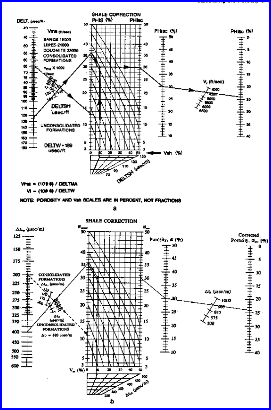
Chart for Estimating Shale Corrected Sonic Porosity
Use the compaction correction only if CDTSH
> 100 (for English units) or CDTSH > 328 (for Metric units).
In western North America, this is normally required when above
3,000 - 4,000 feet (900 - l,200m).
KS is in the range 0.7 to 1.0 depending on gas density invasion
and local experience. It can be derived by comparing the calculated
porosity with the true porosity from cores or density neutron
crossplot methods.
Use gas correction only if PHIS is too high compared to other
sources, only if the zone is clean and does not need shale corrections,
and if gas is known to be present. The need for this correction
is rare. It is very unlikely that a gas correction will be needed
in shaly sands since invasion should be relatively deep.
Another way of making gas corrections is to change DELTW to a higher value, representing the travel time of sound
in a mixture of gas and water. This value depends on water saturation
in the invaded zone, pressure, temperature and gas compressibility.
Values in the range of 600 usec/ft (1900 usec/m) at shallow depths
to 300 usec/ft (950 usec/m) at 6000 feet (2000 meters) are recommended
as a starting point.
KCP can be calculated if true porosity of a clean zone is known
from core, neutron, or density log data:
8: KCP = PHIS / PHItrue
Where:
KCP = compaction factor (fractional) (usec/ft or usec/m)
PHIS = sonic log porosity in clean sand (fractional)
PHItrue = actual porosity in clean sand from core or density data
(fractional)
NUMERICAL EXAMPLE:
1. Wyllie Method - Shaly Sand
DTC = 300 usec/m
DTCSH = 328 usec/m
DTCMA = 182 usec/m
DTCW = 616 usec/m
Vsh = 0.33
KCP = 1.0
Therefore compaction correction is not needed.
PHIS = (300 - 182) / (616 - 182) / 1.0 = 0.27
PHISSH = (328 - 182) / (616 - 182) / 1.0 = 0.34
PHIsc = 0.27 - 0.33 * 0.34 = 0.16
PHIsc is not too high, and no gas is known to be present. Hence,
no gas correction is made.
2. Wyllie Method - Clean Gas Sand
DTC = 380 usec/m
DTCSH = 328 usec/m
DTCMA = 182 usec/m
DTCW = 616 usec/m
Vsh = 0.0
KCP = 1.0
PHIS = (380 - 182) / (616 - 182) / 1.0 = 0.46
PHISSH = (328 - 182) / (616 - 182) = 0.36
PHIsc = 0.46 - 0.0 * 0.36 = 0.46
PHIsc is too high due to gas effect - assume KS = 0.75
PHIsc = 0.75 * 0.46 = 0.33
3. Wyllie Method - Un-compacted Sand
DTC = 375 usec/m
DTCSH = 460 usec/m
DTCMA = 182 usec/m
DTCW = 616 usec/m
Vsh = 0.0
KCP = 460 / 328 = 1.40
PHIsc = PHIS = (375 - 182) / (616 - 182) / 1.40 = 0.31
No gas correction is required.
No shale correction is required.
Fluid Travel Time Values
The acoustic wave from a sonic log travels in the rock near the wellbore face. The pores contain mostly mud filtrate with some
of the original formation fluids (formation water with or
without oil or gas). We generally assume DTCW = 656 usec/m for
fresh water mud filtrate and DTCW = 616 usec/m in saturated salt
water mud filtrate (200 usec/ft and 188 usec/ft respectively, in
English units. However the chart below show that DTCW could be
as low as 168 usec/ft in a saturated CaCl mud system.
Some mud systema use KCl to reduce shale erosion. These are
still relatively fresh water muds compared to saturated CaCl
muds, so the DTCW will still be close to, but less than, the
fresh water value. Mud sytems with seawater makeup have a
salinity of 20,000 to 30,000 ppmso DTCW should about 10% less
than the fresh water value. Saturated NaCl mud may be used while
drilling through salt beds, so the lower limit of DTCW should be
used as a starting point.
Barite weighted muds are usually an emulsion with fresh water
and DTCW varies only slightly wih mud weight.
In oil base muds, invasion is seldom an issue so DTCW depends on
the salinity of the formation water and the hydrocarbon density.
All of this means
that you may need to tinker with DTCW, as well as matrix and shale
terms, to help get a good calibration to core porosity.
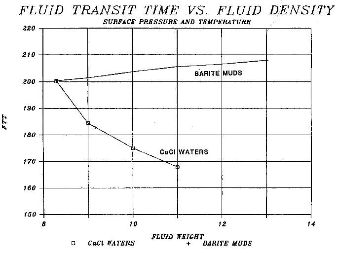
DTCW usec/ft (vertical axis) versus mud weight
for CaCl and barite weighted mud systems
Porosity From the Sonic Log (Hunt-Raymer Method)
The Hunt-Raymer method is a newer formula which is a non-linear
calibration of observed porosity versus log response data. It
should be used in clean sands and carbonates only, or log data
may be corrected for shale first. It can be used in un-compacted
sands without the compaction correction described in the Wyllie
method given above. The algorithm is derived from the following
empirical relationship:
11:
VELOG = VELMA * ((1 - PHIe) ^ 2) + VELW
* PHIe
This can be solved for porosity in the following way:
Calculate sonic log reading corrected for shale:
12: DTC1 = DTC - Vsh * (DTCSH - DTCMA)
Calculate sonic porosity
13: C = DTCMA / (2 * DTCW)
14: PHIShr = 1 - C - (C ^ 2 - DTCMA / DTCW + DTCMA / DTCc)
^ 0.5
Where:
C = intermediate term
DTC = sonic log reading in zone of interest (usec/ft or usec/m)
DTC1 = sonic log reading corrected for shale (usec/ft or usec/m)
DTCMA = sonic log reading in l00% matrix rock (usec/ft or usec/m)
DTCSH = sonic log reading in l00% shale (usec/ft or usec/m)
DTCW = sonic log reading in 100% water (usec/ft or usec/m)
PHIShr = porosity from sonic log by Hunt-Raymer method (fractional)
VELOG = sonic velocity log reading (ft/sec or m/sec)
VELMA = sonic velocity log reading in 100% matrix (ft/sec or m/sec)
VELW = sonic velocity log reading in 100% water (ft/sec or m/sec)
Vsh = shale volume (fractional)
COMMENTS:
A graphical solution for the Hunt-Raymer method, with no shale
correction, is given in BELOW.
Sonic Log Porosity from Hunt-Raymer Method (curved lines) and
Wyllie Method (straight lines)
- Shale Corrections Are Required Before Using This Graph.
Although the original paper does not discuss shale corrections,
they are essential. Gas corrections similar to those used in the
Wyllie method can be used if needed. The answer porosity will
be too high in gas if the corrections are not made. The method
is not universally applicable and should be tested in each area
before use.
Another way of making gas corrections is to change DELTW to a higher value, representing the travel time of sound
in a mixture of gas and water. This value depends on water saturation
in the invaded zone, pressure, temperature and gas compressibility.
Values in the range of 600 usec/ft (1900 usec/m) at shallow depths
to 300 usec/ft (950 usec/m) at 6000 feet (2000 meters) are recommended
as a starting point.
NUMERICAL EXAMPLE:
1. Hunt-Raymer Method - Shaly Sand
DTC = 300 usec/m
DTCSH = 328 usec/m
DTCMA = 182 usec/m
DTCW = 616 usec/m
Vsh = 0.33
KCP = 1.0
DTC1 = 300 - 0.33 * (328 - 182) = 251 usec/m
C = 182 / (2 * 616) = 0.147
PHIShr = 1 - 0.147 - (0.147 ^ 2 - 182 / 616 + 182 / 251) ^ 0.5
= 0.18
2. Hunt-Raymer Method - Clean Gas Sand
DTC1 = 380 - 0.00 * (328 - 182) = 380 usec/m
C = 182 / (2 * 616) = 0.147
PHIShr = 1 - 0.147 - (0.147 ^ 2 - 182 / 616 + 182 / 380) ^ 0.5
= 0.40
Porosity is too high due to gas effect - assume KS = 0.80.
PHIsc = 0.80 * 0.40 = 0.32
3. Hunt-Raymer Method - Un-compacted Sand
DTC1 = 375 - 0.33 * (460 - 182) = 375 usec/m
C = 182 / (2 * 616) = 0.147
PHIShr = 1 - 0.147 - (0.147 ^ 2 - 182 / 616 + 182 / 375) ^ 0.5
= 0.39
This result is a little high compared to the more conventional
method.
Porosity From the Dipole Shear Sonic Log (Wyllie
Method)
The
newer sonic logs record shear travel time as well as the compressional
travel tine. The compressional data is processed as discussed
above under the Wyllie and Raymer-Hunt methods. Shear travel time
can be used in the Wyllie equation, using fictitious values for
fluid travel time. There is very little fluid effect on shear
data so there is no gas correction.
Calculate total sonic porosity
15: PHIS_S = (DTS - DTSMA) / (DTSW - DTSMA)
Correct sonic porosity for shale
16: PHISSH_S = (DTSSH - DTSMA) / (DTSW - DTSMA)
17: PHIsc_S = PHIS_S - Vsh * PHISSH_S
Where:
DTS = shear sonic log reading in zone of interest (usec/ft or
usec/m)
DTSMA = shear sonic log reading in l00% matrix rock (usec/ft
or usec/m)
DTSSH = shear sonic log reading in l00% shale (usec/ft or usec/m)
DTSW = (fictitious) shear sonic log reading in 100% water (usec/ft
or usec/m)
PHIS_S = porosity from shear sonic log before shale correction
(fractional)
PHIsc_S = porosity from shear sonic log by Wyllie method (fractional)
PHISSH_S = apparent shear sonic porosity of 100% shale (fractional)
Vsh = shale volume (fractional)
COMMENTS:
Shear travel time is more sensitive to porosity than compressional
data.
No gas correction is needed.
The measurement can usually be made through casing so this is
a good choice for cased hole logging.
There is no record of a compaction correction being applied, but
this may be needed. Comparison to core porosity or density neutron
crossplot porosity will indicate when such a correction is needed.
|
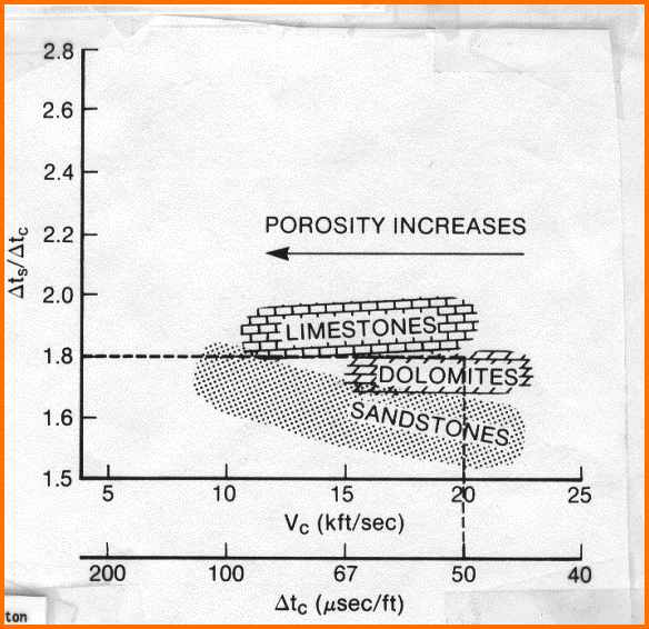
Table 1: KS8 – DTS / DTC Multiplier |
|
Coal |
1.9 to 2.3 |
|
Shale |
1.7 to 2.1 |
|
Limestone |
1.8 to 1.9 |
|
Dolomite |
1.7 to 1.8 |
|
Sandstone |
1.6 to 1.7 |
Shear travel time for fluid is a fictional value
(pseudo-travel time) equal to Vp/Vs ratio times compressional travel
time. Vp/Vs ratio can be estimated by:
18:
KS8 = SUM (Vxxx * (DTS/DTCmultiplier))
Where:
Vxxx = volume of each mineral present, normalized so that SUM(Vxxx) = 1.0
Where:
(DTS/DTCmultiplier) = Vp/Vs ratio for a particular mineral (Table 1)
|
RECOMMENDED PARAMETERS - SHEAR TRAVEL TIME |
|
|
English - usec/ft |
Metric - usec/m |
|
DTSSH |
96 -
240 |
490 -
770 |
|
DTSW
fresh water |
350
** |
1280
** |
salt water
|
340
** |
1200
** |
|
DTSMA |
|
|
|
Granite |
80.0 |
262 |
|
Quartz |
88.8 |
291 |
|
Limey sandstone |
88.9 |
292 |
|
Limestone |
89.9 |
294 |
|
Limey dolomite |
82.3 |
270 |
|
Dolomite |
74.8 |
245 |
|
Anhydrite |
85.0 |
280 |
|
Coal |
152+ |
500+ |
**
Set equal to Vp/Vs times compressional sonic value
Porosity from Vp^2 / Vs^2 (Biot-Gassmann)
Method
The Biot -- Gassmann equations can
be rewritten to derive porosity from the Vp / Vs ratio (the ratio of
compressional to shear velocity) using known values of matrix
velocity (derived from standard travel time (slowness) data and the
log readings from compressional and shear sonic logs. The equation
set is as follows (Krief, 1987, updated by Michel Krief, via email,
Aug 2015):
Convert travel time to velocity
18: Vp = 10^6 / DTC
19: Vs + 10^6 / DTS
Solve the following equation set for PHIt
20: Beta = (1 - Phit)^(BetaExp / (1 - Phit))
21: BetaS = (1 - Phit)^(BetaSExp / (1 - Phit))
22: 1 / Mb = (Beta - PHIt) / Km + (PHIt / Kf
23: DENS * Vp^2 = DENSMA * (VPMA^2) * (1 - Beta)
+ (Beta^2) * Mb
24: DENS * Vs^2 = DENSMA * (VSMA^2) * (1 .
BetaS) *** note the use of BetaS ***
Where:
BetaExp = 3.0 by default (grainstone), with a range up to 100 (mudstone)
BetaSExp = 3.0 by default (grainstone), with a range up to 100 (mudstone)
Beta = Biot's coefficient (ALPHA was used elsewhere in this Handbook for
Biot's constant)
BetaS = Gassmann's coefficient
Mb = Biot's modulus
DENS = density log reading
DENSMA = matrix rock density
Vp = compressional velocity from travel time log
VPMA = matrix rock compressional velocity
Vs = shear velocity from travel time log
VSMA = matrix rock shear velocity
Km = bulk modulus of matrix rock
Kf = bulk modulus of pore fluid
Beta (Biot coefficient) is for the calculation of bulk modulus,
BetaS (Gassmann coefficient) for the calculation of the Shear
modulus. Beta and BetaS are not necessarily equal. BetaExp and
BetaSExp are coefficients which may be called Biot-Krief exponent
and Gassmann-Krief exponent.
COMMENTS:
This set of four non-linear equations
must be solved for PHIt in terms of Vs^2 and Vp^2. Probably the
solver in Excel will do it, but I haven't tried it. By using volume
weighted averages of shale and matrix rock properties for the matrix
terms, you can replace PHIt with PHIe. Kf can be set to account for
gas, oil, or water.
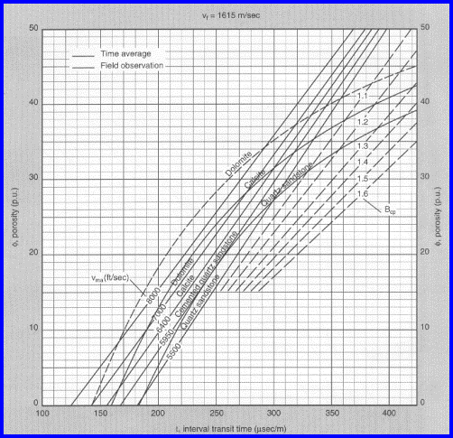
A graph showing the result for
clean rocks is shown below.
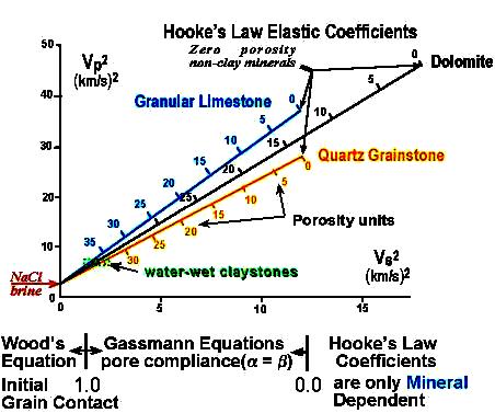
Vp^2 versus Vs^2 for
calculating porosity.. Gas point is very close to the graph origin,
so
slope of lines steepens slightly. Porosity scale on the lines
stretches a bit but matrix points do not move.
SONIC
LOG PARAMETERS (COMPRESSIONAL TRAVEL TIME
)
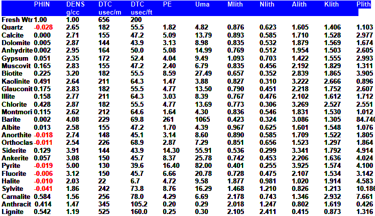
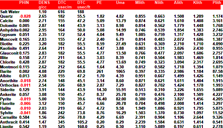
|