The
above relationship must be derived for each particular area by
curve fitting the laboratory data. Some authors have related CEC
to porosity in certain areas, but there is no physical reason
why this should be true, since specific CEC values depend on shale
volume and clay type, and not porosity. The only time this might work is when
porosity is strictly a function of shale volume and there are
no other mineral variations. Others have tried to relate CEC to
some other log data, such as the SP (which of course is a shale
indicator), with limited success. CEC data from laboratory
measurements are now routine. Where:
mineral analysis based on elemental capture spectroscopy (ECS) log: Reference: Good CEC data is still hard to come by. CEC measured on core and sample chips often do not correlate well with either effective porosity or shale content, most likely due to the fact that more than one clay mineral is present, each in varying proportions. Thus a pragmatic fit of CEC to a log derived porosity or shale volume is usually necessary. This field specific approach is commonly applied by those who insist on using the Waxman-Smits approach even when the lack of data does not support its use. Some analysts use density porosity (PHID), uncorrected for shale, to predict CEC. Some use PHID in the saturation equations instead of PHIe. Others call PHID the “total porosity”, which is wrong, since the standard definition of total porosity is (PHIN + PHID) / 2. These terminology problems stem from shortcuts used in specific areas before sophisticated computer programs made it easy to do better work. Unfortunately, younger analysts learn the tricks of the trade from older analysts who have long forgotten that the shortcut was ever taken.
If
Qv or Vsh were higher the saturation would be lower. |
|
||
|
Page Views ---- Since 01 Jan 2015
Copyright 2023 by Accessible Petrophysics Ltd. CPH Logo, "CPH", "CPH Gold Member", "CPH Platinum Member", "Crain's Rules", "Meta/Log", "Computer-Ready-Math", "Petro/Fusion Scripts" are Trademarks of the Author |
|||

|
||
| Site Navigation | WATER SATURATION WAXMAN SMITS MODEL | Quick Links |
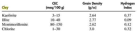 An
alternative is to calculate CEC from a clay
An
alternative is to calculate CEC from a clay