|
 Seismic Inversion and Synthetic Sonic Logs
Calibration
of seismic attributes to ground truth is still an emerging science.
No single attribute (eg. amplitude, frequency content, attenuation,
compressional or shear velocity, or acoustic impedance) can be
related directly to a specific rock property (eg. porosity, lithology,
hydrocarbons). However, geoscientists have found that one or more
attributes may predict some reservoir property in a particular
project. Trial and error is the only way to find out what works.
One
of the most successful is the use of Poisson's Ratio to indicate
the presence of porosity or gas. This requires close calibration
to log data - many early studies obtained impossible numbers for
Poisson's ratio, indicating poor quality inversion of the compressional
or shear data into velocity. A successful example is shown later
in this Chapter.
When
attributes are used to locate hydrocarbons, they are often called
direct hydrocarbon indicators or (DHI). Bright spots and dim spots
(amplitude anomalies on conventional seismic displays) were the
earliest form of DHI. Many bright spot studies failed because
many different factors create the amplitude variation. Log
modeling
will show what kind of amplitude to expect for different reservoir
conditions.
DHI
is no longer a popular term because hydrocarbon indicators are
really porosity or lithology indicators, with a major contribution
from gas if it is present. The difference in acoustic and density
properties between oil and water is very small and well below
the noise level of even the best logs, let alone seismic.
The
same story is true of amplitude versus offset (AVO) anomalies.
Models are the only way to see what a particular AVO output might
mean. Examples are shown below.
Wavelet processing of modern seismic field data yields
results containing much more information than is found on
conventionally processed data. These sections are usually
called wide band or broad band sections. Yet the results may
not bring joy to the average interpreter due to the noisy
appearance of the data.
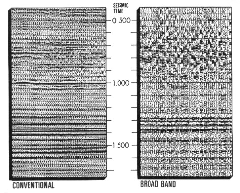
Normal and broadband seismic data
Instead
of simplifying the interpretation, the additional detail appears
to mask the more obvious features on the conventional section
and make the horizons more difficult to map. In fact, some of
the principal markers on the conventional section practically
disappear on the broad band section, while others appear to be
displaced in time.
The
broad band data approaches the response of the reflection coefficients
and more accurately represents the acoustic impedance changes
in the rock sequence. However, if the broad band data is to be
used, some other means, other than the seismic wiggly trace, must
be found to display it in a manner which can be adapted to routine
interpretation.
One
way to do this is to rearrange the reflection coefficient
equation to solve for velocity, and display these velocities
versus time or depth just like a sonic log. This requires
the first velocity to be known, but thereafter all others
can be derived by applying the formula in succession to each
reflection coefficient.
The acoustic impedance from inversion of seismic
data is:
_____1:
Zp2 = Zp1 * (1 + Refl1) / (1 - Refl1)
If density is assumed based on lithology, the inversion can produce velocity
instead of acoustic impedance. Inversion can be applied to both compressional
and shear seismic data.
 This
equation suffers from progressive errors as successive layers
are computed. I wrote a program to do this calculation on a TIAC
in 1966 but it failed miserably - the data was too low in bandwidth
and I hadn't thought of finding the low frequency component from
nearby sonic logs. Roy Lindseth produced the first commercial
synthetic sonic logs around 1969 in Calgary. This
equation suffers from progressive errors as successive layers
are computed. I wrote a program to do this calculation on a TIAC
in 1966 but it failed miserably - the data was too low in bandwidth
and I hadn't thought of finding the low frequency component from
nearby sonic logs. Roy Lindseth produced the first commercial
synthetic sonic logs around 1969 in Calgary.
The
problem is reduced by filtering the results and stretching or
squeezing to fit real, filtered sonic logs.
If
this procedure is used to create an approximation of reflection
coefficients from seismic data, and is expected to correlate to
a real sonic log, some compensation must be made for the effects
of density. Acoustic impedance is the product of velocity and
density, so an inverted seismic trace is an acoustic impedance
log rather than a sonic log. Fortunately, velocity is, to some
degree, a linear function of acoustic impedance.
The inverted data can be corrected accordingly.
Filtered
sonic log 
A
serious constraint to inversion is the limited bandwidth caused
by filtering which may occur through the system. Both the earth
(subsurface) and electronic filters reduce frequency content.
A sonic log has a very broad frequency bandwidth, extending from
DC to approximately 1000 Hz. Current field practice and equipment
limits the low end of the seismic spectrum to about 8 to 10 Hz
while the natural filter of the earth eliminates frequencies much
over 100 Hz, depending upon the depth. Careful stacking and de-convolution
will recover a good portion of the spectrum, often almost doubling
the bandwidth of about 50 Hz on conventional data.
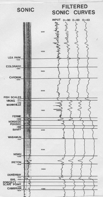
A
sonic log can be filtered to demonstrate the loss of resolution
caused by high cut filtering (Figures 24.03 and 24.04). The effect
is roughly analogous to logging with a very long tool spacing,
which decreases the resolution of the log by smoothing out high
frequency information. A seismic trace of the same frequency will
have resolution no better than the log.
Low frequency content of a sonic log
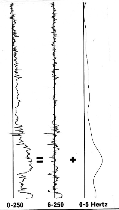
Separating low and high frequency components
on a sonic log
Of greater concern are low frequencies, which are usually lost
through geophone response or band-limiting by the recording instruments.
Frequencies
lost from the spectrum cannot be restored by de-convolution. Depending
upon the geophones used and the seismic system response, frequencies
below 5 to 10 Hz will be irrevocably lost from the spectrum. The
absence of these frequencies is very serious, since they carry
the basic velocity structure of the log.
 In
fact, a sonic log can be considered in terms of a low frequency
carrier function modulated by higher frequencies. The effect is
illustrated above, where 6 Hz has been chosen as a crossover
frequency to separate a time integrated sonic log into its low
frequency and high frequency components. The sum of the two components
yields the original sonic log. In
fact, a sonic log can be considered in terms of a low frequency
carrier function modulated by higher frequencies. The effect is
illustrated above, where 6 Hz has been chosen as a crossover
frequency to separate a time integrated sonic log into its low
frequency and high frequency components. The sum of the two components
yields the original sonic log.
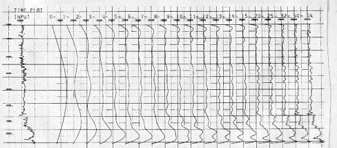
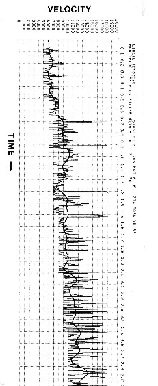
The
first step in generating the low frequency data is to extract
reliable vertical velocity information from stacking velocities.
 A computer can pick a great number of sample points, which then
can be statistically evaluated. The example at the left illustrates
the results of a constant velocity analysis machine picked each
8 ms. The results are extremely erratic and apparently of little
use, but application of a 7 Hz low pass filter yields a smooth
continuous low frequency velocity curve. A single curve of this
type probably contains residual errors, but several curves, closely
spaced, can be averaged to produce more reliable results. The
average velocities are then converted to interval velocities by
ray path modeling. A computer can pick a great number of sample points, which then
can be statistically evaluated. The example at the left illustrates
the results of a constant velocity analysis machine picked each
8 ms. The results are extremely erratic and apparently of little
use, but application of a 7 Hz low pass filter yields a smooth
continuous low frequency velocity curve. A single curve of this
type probably contains residual errors, but several curves, closely
spaced, can be averaged to produce more reliable results. The
average velocities are then converted to interval velocities by
ray path modeling.
 Low frequency component of synthetic sonic log derived from
a velocity analysis of seismic data Low frequency component of synthetic sonic log derived from
a velocity analysis of seismic data
With
the low frequency velocity information developed, the density
corrected, inverted seismic data above the crossover frequency
can be summed with the velocity data below the crossover to yield
the synthetic sonic, scaled in time and velocity. This log can
be easily converted to scales of depth and interval transit time
and then compared to real sonic logs.
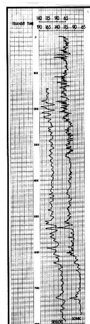
This
is the procedure used to obtain the synthetic sonic log, generally
termed Seislog, shown at the right. It has been plotted together with a borehole
compensated sonic log for comparison. The vertical
scale is depth, and the horizontal scale is microseconds per foot,
both normal parameters for sonic logs. The seismic data has been
converted into the geological domain. It is expressed in terms
familiar to a geologist and is directly correlative to conventional
geological data.
Comparison of filtered sonic log and seismic inversion
trace
It would be natural to calibrate the synthetic sonic logs at
each well along the seismic lines, and then extend the work to
all seismic traces along the lines. This creates synthetic sonic
log cross sections. The process is called seismic inversion, and
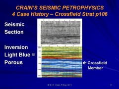
is covered in more detail on the next Chapter. A sample inverted
seismic section is shown below
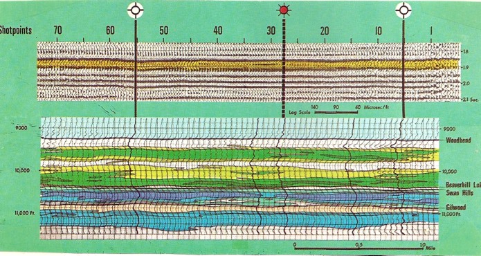
This example shows a cross section of synthetic sonic log
traces calibrtaed at 3 well bores along the seismic line. This
product is called a seismic inversion.
|