|
 Statistical
Curvature Analysis Techniques - SCAT Diagrams
Statistical
Curvature Analysis Techniques - SCAT Diagrams
Traditional dipmeter analysis techniques used for structural
analysis involve pattern recognition on the dip arrow, or
tadpole, plot.
While this approach can be learned with study and practice, there
are other approaches that can be applied.
Alternatives to the conventional arrow plots have been proposed,
mainly because of the effects of statistical variations and ambiguous
patterns which sometimes make arrow plots hard to use.
The most
successful technique is called statistical curvature analysis,
better known as SCAT. The method lends itself to interactive computer
programming, and was described by C.A. Bengtson in "Statistical
Curvature Analysis Techniques for Structural Interpretation of
Dipmeter Data", published in AAPG Bulletin in 1981. The paper
was also printed in Oil and Gas Journal, June 1980 and in Geobyte,
May 1988.
Microcomputer
programs for analyzing dipmeter data in this way were presented
by Robert Elphick in the May 1988 and March 1989 issues of Geobyte.
These programs do not seem to be available from the major service
companies.
SCAT
is based on four unfamiliar, but empirically well verified, geometric
concepts:
1. structural curvature
2. transverse and longitudinal structural directions
3. special points on dip profiles
4. dip isogons or trend lines
Flat
or dipping planes have zero or planar curvature. Horizontal or
plunging folds have one degree of curvature. Doubly plunging folds
have two. Drag and rollover on faults have structural curvature
and can be analyzed in the same way as folds. Illustrations of
typical surfaces and their dip angle vs dip azimuth plots are
shown in below.
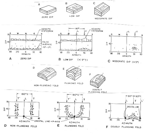
Dip angle vs azimuth plots - basic shapes
The
obvious difference between SCAT and the conventional approach
is that SCAT uses the dip angle vs dip azimuth plot plus four
other machine plotted dip vs depth displays, whereas the conventional
method relies on an all purpose display, the arrow plot, augmented
by azimuth frequency plots over selected intervals.
The
five plots used in SCAT are:
1. dip angle vs dip azimuth
2. dip azimuth vs depth
3. dip angle vs depth
4. transverse section dip angle vs depth
5. longitudinal section dip angle vs depth
The
patterns on dip angle vs dip azimuth plots may be simple or complex.
However, they are usually simpler and never more complex than
patterns on arrow plots.
Arrow
plots show complex patterns when a well crosses a crestal plane,
but transverse dip component plots show smooth trend lines that
cross the zero dip axis. Because angle of dip on an arrow plot
is neither positive nor negative, there is no chance for a negative
scatter to cancel positive scatter in a flat dip situation. Therefore,
a zone of zero dip is falsely perceived as a zone of a few degrees
average dip with varying dip azimuth. On a dip component vs
depth plot, however, half of the points will fall to the right
of the zero dip axis and half to the left, correctly indicating
zero average dip.
SCAT
resolves the data into mutually perpendicular transverse and
longitudinal (or T- and L-direction) components, using the dip
rotation arithmetic described elsewhere in this Handbook
The T-direction is defined as the direction of cross section through
the well that shows the greatest structural change, and the L-direction
as the direction that shows the least structural change. These
directions are chosen from the locations of the maximum and minimum
dip angle scatter on the dip angle vs azimuth plot, marked T and
L. They are usually orthogonal directions and
can be picked by eye or by statistical analysis.
Average
L-direction component of dip is zero for planar and nonplunging
fold settings and equal to the angle of plunge for plunging fold
settings. On plunge reversal settings the average L-direction
component of dip shows a reversal of dip (and hence plunge) with
depth. The only exceptions occur in wells cut by cross faults.
However, longitudinal dip component plots may show considerable
scatter in zones of steep dip.
The
shape of the statistical trend line on a transverse dip vs depth
plot defines the bedding curvature on a transverse cross section.
A trend line conforming to constant dip indicates planar curvature.
A smoothly curved trend line with no bends or reversals indicates
uniform or smoothly varying curvature, whereas a trend line with
bends or reversals will show one or more of eight mathematically
definable patterns or special points.
Six
of these points serve to locate and identify structural surfaces
(axial planes, kink planes, inflection planes, secondary inflection
planes, minimum curvature planes, and zero strain boundaries)
that intersect the well, and two serve to locate dip-slip faults,
distinguishing faults that dip to the right from faults that dip
to the left.
Finally,
it should be stressed that SCAT has the capacity to find the bearing
and plunge of crestal and trough lines of folds, the strike and
dip of crestal, axial, and inflection planes of folds, and the
strike and direction of dip of dip-slip faults. Dip arrow plots
do not handle this function very well.
The
concept that there are only a few types of structural curvature
greatly simplifies interpretation. Beds are either planar or curved;
if planar, the beds are either horizontal or dipping. A zero dip
homocline shows no structural change in any direction and hence
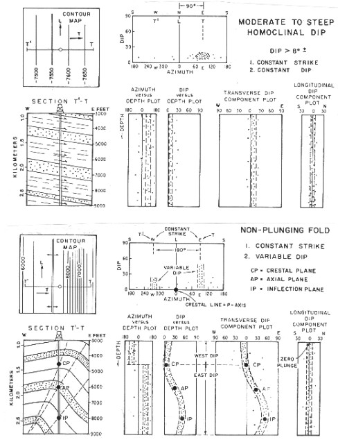
has no T- or L-directions. In the low
and higher homoclinal dip settings (Figures 32.02 bottom, 32.03
top) the T-direction parallels the dip and the L-direction parallels
the strike. Patterns on T, L, and azimuth vs depth plots are vertical
and a maximum density of points will occur at the average regional
dip on the dip vs azimuth plot.
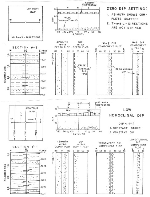
SCAT plots for zero dip setting
SCAT plots for homocline and fold settings
If
the beds are curved, they are either singly or doubly curved.
If single curved, their crestal or trough lines are either horizontal or plunging at a constant angle. In either situation, the T-direction is perpendicular
to the crestal or trough lines and the L-direction is parallel.
The L component graph will be vertical. The others will be curved.
The depth of crestal, axial, and inflection planes are found by
observation of the bends in the trends.
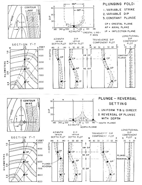
SCAT plots for plunging fold settings
If the beds are doubly curved, their structure contours are either
elliptical or circular in plan. If elliptical,
their geometry can be approximated by two singly curved plunges
joined by a non-plunging central sector, in which case the T-direction
is perpendicular to the crestal or trough lines and the L-direction
parallels the long dimension. If the structure contours are circular,
the transverse directions will converge radially toward the center,
and the longitudinal directions will be disposed circumferentially
around the center. L-component patterns also have bends.
SCAT
plots through faults show the pattern of the structural setting
around the fault and the drag is superimposed on it. The fault
usually creates a cusp on the transverse dip section, pointing
in the direction of the dip of the fault for normal faults and
opposite to the dip for reverse faults. (Figures 32.05 and 32.06).
The drag patterns are quite distinctive on SCAT plots and help
to differentiate faults from folds. Rollover creates a half cusp
pattern. These patterns are similar to red and blue patterns seen
on dip arrow plots of faults.
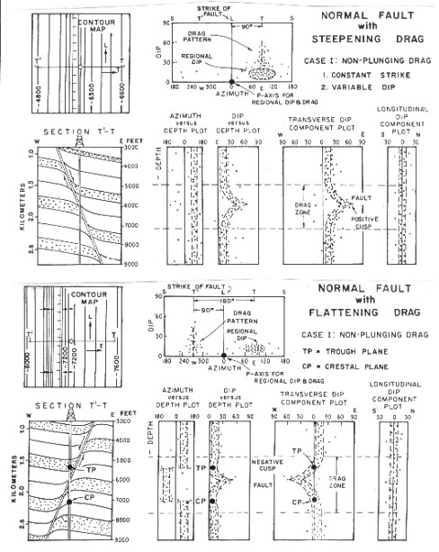
SCAT plots for fault settings
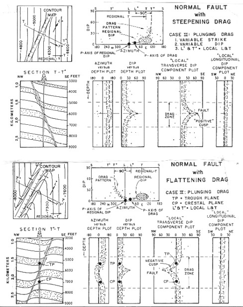
More SCAT plots for fault settings
|