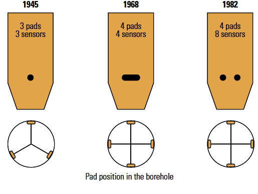
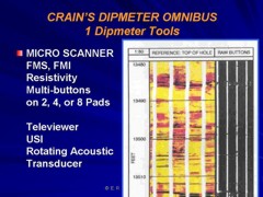
This page describes dipmeter logs profiles, in the order of their appearance over the years. This presentation style provides insights into tool evolution, and a specific tool’s capabilities and limitations. You will find most these tool types in your well files – here’s your chance to learn more about them.
In the beginning, there were no dipmeters. Dip magnitude and direction
of rock strata was assessed by knowing the subsea elevation of
a distinctive rock layer in three or more wells which were closely
spaced. The equation of a plane is defined by the X, Y, and Z
coordinates of three points, so the elevations and well locations
were sufficient data to define dip. Subsurface mapping of clearly
defined formation markers is widely used today to estimate both
regional and local dips.
Conventional dipmeters work in conductive muds in open hole and specialized
special tools are available for oil based mud
systems. They do not work in cased holes.
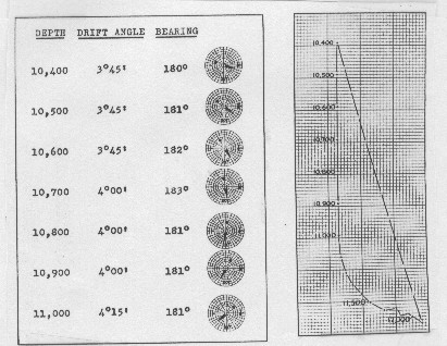
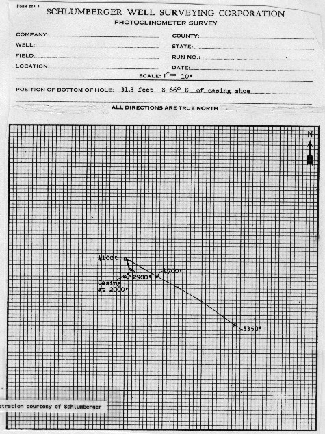
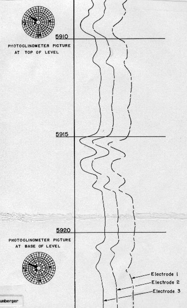
The
balance of the data came from a photoclinometer survey taken at
stations near the top and bottom of the recorded intervals of
the dipmeter curves. A schematic example of the concept is shown
below. The photoclinometer consisted of a magnetic compass,
a ball bearing in a graduated curved dish, and a camera that photographed
these components on demand.
This sounds simple. However, the magnitude of dip which is of interest in exploration is from a fraction of 1 degree to vertical. This poses serious constraints on tool design and data analysis. For example, a regional dip of about 50 ft/mile is equivalent to 1/2 degree dip. Local structure or drape over deeper erosional surfaces may modify this dip to flat or 1/2 degree in another direction. In some areas this is significant and could define the trapping mechanism. The dipmeter device, the recording process, and the curve correlation methods must have sufficient resolution to enable us to see this small difference. A bed dipping at 1/2 degree across a 9" borehole will be less than l/10 inch higher on one side of the hole than on the other. The displacement between curves will be less than 0.1 inches if recorded at 12 inches per foot of borehole. If recorded at 5 inches per hundred feet, a normal detail logging scale, this displacement would be only 0.0004 inches on the film. As a result, scales of 60 inches per 100 feet were used. Now the 1/10 inch displacement is represented by 0.005 inches - a measurable distance on the film. Due to the relatively round shape of the SP curve at most bed boundaries, this level of resolution was not achieved with the SP dipmeter. Moreover, the tool was useless in carbonates where SP does not develop well. The only dips presented were those from major bed boundaries where dip was steep enough to be obvious. Although
the SP dipmeter was abandoned quickly in favour of three resistivity
curves, the photoclinometer survived well into the 1960's as a
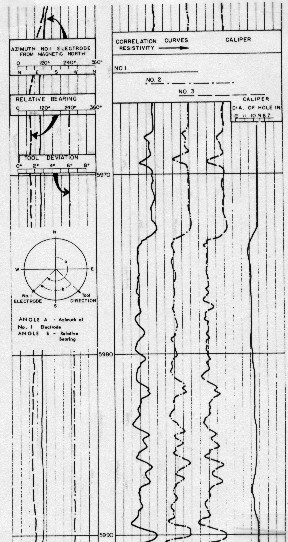
directional survey tool. A sample is shown below. In
addition to the photographs of the compass and deviation ball,
typed listings of computed results and a plan of the well track
were presented. Since the well bore
often deviated, without any help from the drilling crew, to keep
the bit perpendicular to the formation dip, the directional survey
data was sometimes used as a guide to dip.
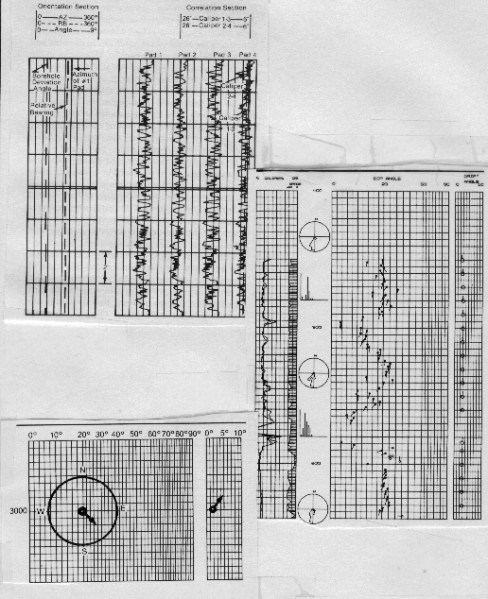
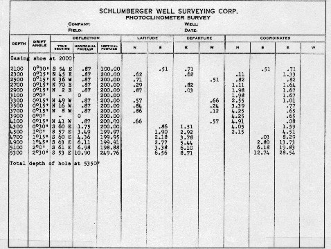
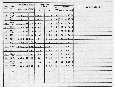
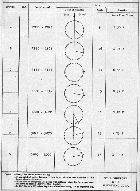
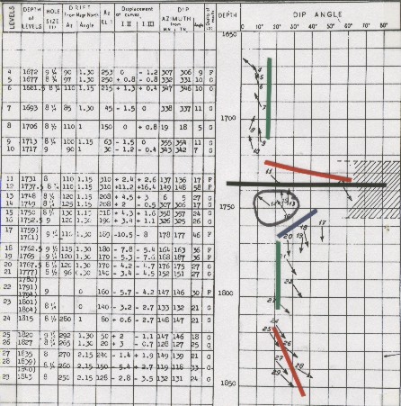
Typical computed results from the SP or resistivity dipmeter are shown below. Although rare, examples can be found in files for wells drilled in the 1940's.
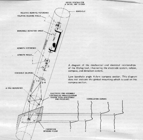
Orientation data was recorded simultaneously and continuously with a device called a poteclinometer. Poteclinometer is a contraction of the word potentiometer (a variable resistor) and inclinometer - this word sounds a lot like the earlier photoclinometer. Directional output from this device is an electrical signal instead of photographs. Data consisted of hole deviation angle, relative bearing (which describes the angle to the high side of the hole from pad number one), and the azimuth (which describes the angle between magnetic north and pad number one). This is sufficient data to orient the dip azimuth and the direction of hole deviation. The algebra is described later in this Chapter. This eliminated the need to stop the tool to take pictures with the photoclinometer. Directional surveys run with this equipment were also more accurate, but considerably more expensive. The optical comparator was also developed during this period. This increased dip accuracy further by reducing errors in measuring the offset between traces. The computed data was presented in the same tabular and graphical fashion as previously , but with considerably higher frequency. However, by 1958, some hardy souls were plotting individual dips as small arrows on a graph of dip magnitude versus depth. The direction of the arrow represented the dip direction relative to a compass rose with north at the top. This was the precursor to the now common arrow plot, sometimes called a tadpole plot, generated by computer. Computer plotting was first seen around 1961.
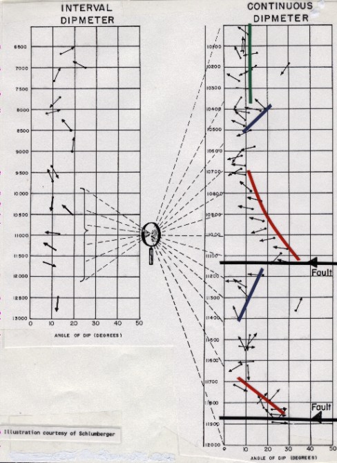
The
first attempts to legitimately use detailed dip data for stratigraphic
evaluation occurred around 1955. An example of the difference
in data quality and quantity between short interval and continuous
data is shown below. The raw data was recorded at 60
inches of log for 100 feet of wellbore, or 1:20 scale, shown half
size below. Literally miles of this photographic paper
was developed, processed, and sifted through the optical comparator
each month. Most of it has deteriorated or been destroyed and
is not available for re-computation.
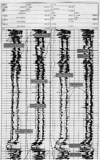
Fortunately, beginning in 1961, dipmeters were recorded on digital magnetic tape, reducing and finally eliminating the need for the detailed paper logs. The offsets between traces were derived by computer correlations, leading to a whole new language: correlation window, step length, search angle, etc.
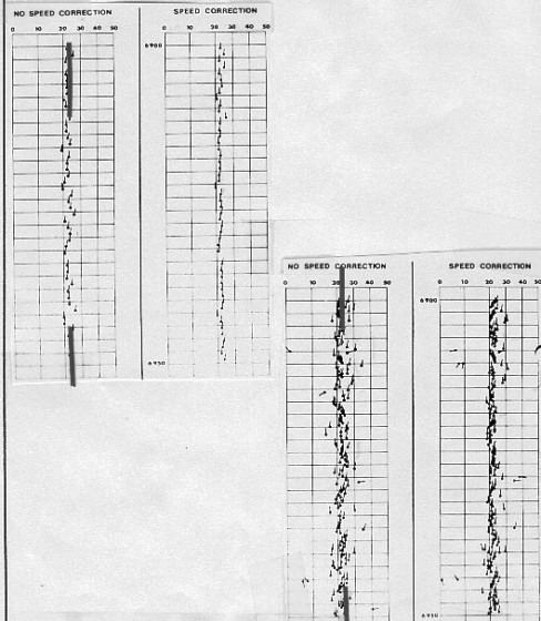
A special "speed button" on one pad provided information to the program to compensate for minor speed differences as the tool moved up the hole. These variations created scatter in the computed results, illustrated below. In addition, a synthetic resistivity curve was generated from the dip curves, to be used as a correlation curve.
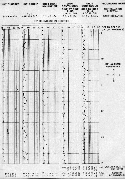
In 1975, secondary computer processing, called CLUSTER (Schlumberger trademark) or SHIVA (Gearhart trademark), were developed to validate the results from the standard program. Other secondary programs were developed to enhance stratigraphic features, notably GEODIP (Schlumberger trademark). These processes are described later. About 1980, three axis accelerometers and three axis magnetometers replaced the magnetic compass, relative bearing, and hole azimuth potentiometers. However the log still presented these three curves, derived now from the solid state sensors instead of the more failure prone electromechanical devices.
Three
dip computation modes are available from the stratigraphic high
resolution dipmeter. The same mathematical algorithms are
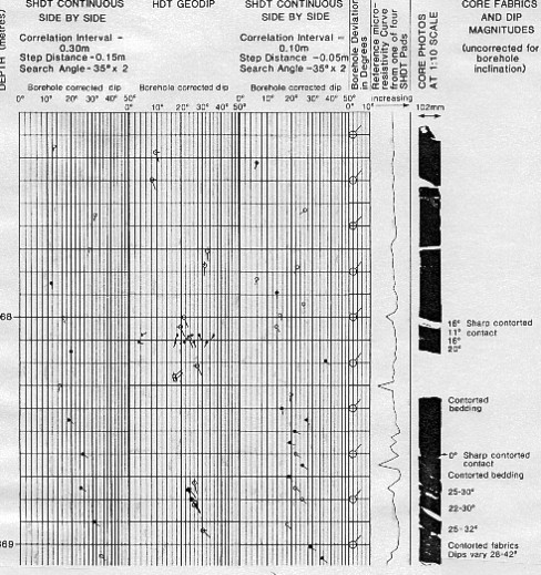
available on resistivity image logs. Second is called Continuous Side by Side or CSB dip correlation using only the individual electrode pairs on each pad. Dip vectors from adjacent electrode pairs are used to define dip. CSB dips respond to short interval, low contrast changes often characteristic of internal layering in clastics, but also will respond to high contrast structural dips. It is very useful for structural dip analysis in high angle apparent dip, greater than 50 degrees. In finely bedded rocks exhibiting cross bedding, considerable detail can be shown if the correlation length and step distance are kept fairly short. Third are pad to pad correlations using a pattern recognition rather than cross-correlation system. This is called Local Dip or LOC dip and responds to non-repetitive events such as erosional surfaces or breaks in the depositional sequence. A comparison of the three modes with normal high resolution dipmeter results is shown below. It is now possible to analyze data with a resolution of a few inches and compare it to core data .
Schlumberger introduced a dipmeter for use in oil-based (nonconductive) mud systems in 1988. It uses micro induction resistivity measurements instead of the usual electrical resistivity pads. A knife blade electrode, or scratcher pad, version is available from several suppliers. In 1989, a 4 arm focused acoustic dipmeter, suitable for both conductive and non-conductive mud, was introduced by Atlas Wireline, with a resolution of about 1 cm.
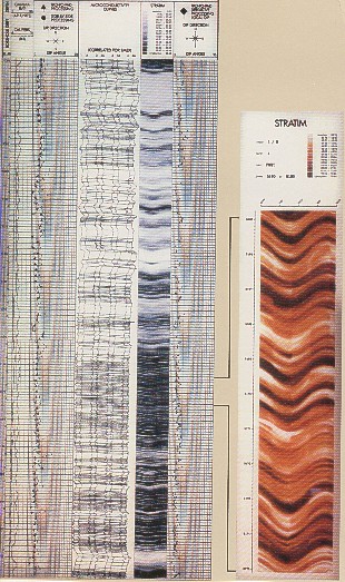
An example is given on the left. The program produces a 360 degree image of the borehole wall by interpolating between the eight resistivity measurements from the eight electrodes on the SHDT pads. Images can be coded in gray scale or colour. Dark gray or dark colour usually represents conductive, often tight shale, beds and light colour resistive, often porous sand, beds. If shales are more resistive than sands (or carbonates), the colour scheme can be reversed to keep shales looking dark.
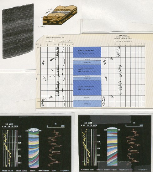
A similar program, called DIPVUE was available from Western Atlas, illustrated below. Here the 3-D image can be rotated in real time to view the artificial "core" from any direction. In addition, most core service companies can provide core photographs and dip logs from core data for comparison with log derived borehole images.
|
|
||
|
Page Views ---- Since 01 Jan 2015
Copyright 2023 by Accessible Petrophysics Ltd. CPH Logo, "CPH", "CPH Gold Member", "CPH Platinum Member", "Crain's Rules", "Meta/Log", "Computer-Ready-Math", "Petro/Fusion Scripts" are Trademarks of the Author |
|||

|
||
| Site Navigation | TOOL PROFILES DIPMETER LOGS | Quick Links |
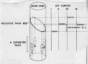 The
geometry of a four pad device is shown schematically at left and the arrangement of tool components
below.
The
geometry of a four pad device is shown schematically at left and the arrangement of tool components
below.