This page describes neutron logs profiles, in the order of their appearance over the years. This presentation style provides insights into tool evolution, and a specific tool’s capabilities and limitations. You will find most these tool types in your well files – here’s your chance to learn more about them.
The first commercial neutron logs were run in 1945 by Lane Wells. They are based on particle physics concepts. Neutron logs emit fast neutrons from a source at the bottom of the tool. The effect of interactions with the rocks and fluids on the neutron flux is measured by detectors above the source on the logging tool. Hydrogen has by far the largest impact, so the tool can be calibrated to represent hydrogen index, which is highly correlated with porosity. So neutron logs are considered to be porosity indicating tools. There are three basic neutron logging instruments
with a chemical neutron source. Each instrument is classified
according to the energy level of the detected particles. Fast
neutrons have energies greater than 100 KeV; epithermal
neutrons have energies above 0.025 eV up to 100 KeV; thermal
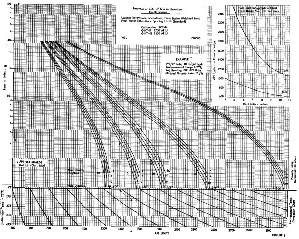
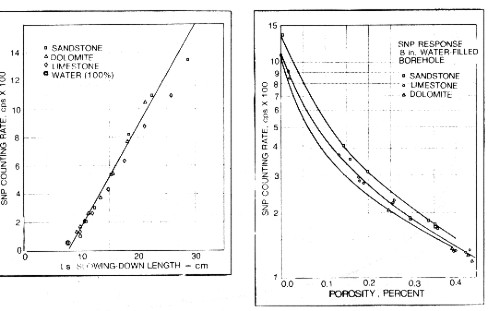
neutrons have an energy of approximately 0.025 eV (at 25 C). The emitted neutrons come from a radium – beryllium or an americium – beryllium source. Radium and americium are natural alpha particle emitters and the alphas eject fast neutrons from the beryllium. With its 433 years half life, the AmBe source output is considered very stable. Approximately 40 x 10^7 neutrons/sec at 4.5 MeV average energy are emitted by the source. When the neutrons are sufficiently slowed down by collisions with the formation, they are captured by the nuclei and a high energy gamma ray of capture is emitted. The gamma ray count rate at the detector is inversely proportional to the hydrogen content of the formation, in a semi-logarithmic relationship. Borehole size and mud weight corrections and calibration to porosity was done by the log analyst. Detectors were Geiger-Mueller gamma ray counters. The source to detector spacing on the older tools was 15.5 inches, giving good statistical accuracy. Longer 18.5” spacing tools became popular because they were more sensitive to porosity but suffered from higher statistical variations. These tools are obsolete and no longer available, but many thousands exist in well files waiting for the serious petrophysicist to use for finding bypassed oil and gas. A large number of charts for specific tools, spacings, borehole conditions and rock types were available from service companies, such as the one shown below. These may no longer be easily found today, and the semi-logarithmic approach described below works well except in very low porosity .
If no appropriate chart exists, or if you don't believe in them, it is expedient to use the "High porosity- Low porosity" method. 1. Select a high porosity point on the log, usually a shale, and assign it a porosity based on offset wells with scaled logs or a local compaction curve. This is PHIHI. 2. Pick the count rate on the neutron log at this point - this is CPSHI, even though it is a low numerical value. 3. Choose a low porosity point on the log. Assign this a porosity value, again based on offset scaled porosity logs or core porosity. This is PHILO. Tight lime stringers or anhydrite are best but you need some imagination if there are no truly low porosity streaks. 4. Pick the corresponding count rate on the log. This CPSLO, even though it is a larger number than CPSHI. 5. Plot these points on semi-log graph paper as shown below. Read porosity for any other count rate from the graph.
To use this plot in a calculator or computer
instead of on a graph:
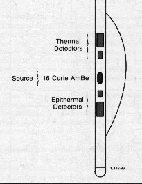
The source and detector are on a skid identical to the density
logging tool. The skid is pressed against the borehole walls,
eliminating most borehole and mudcake effects, except for very
rugose hole conditions.
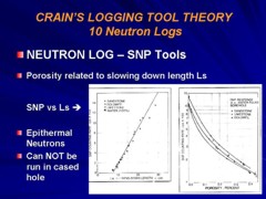
Also shown above is the same count rate data plotted against the calculated slowing down length Ls. A linear best fit is used to describe the correspondence between count rates and slowing down length. At low porosities, there is some lithological effect. Different rocks with the same count rate have different slowing down lengths. Also for some reason, the water point does not fit the line. Fortunately this is not serious as logs are seldom run in zones with more than 45% water. If we know, or can calculate, the slowing down length for neutrons of epithermal energy, in particular rocks, such as calculated in the previous Section, we can enter this value in the graph above and obtain the apparent porosity reading for a real SNP type tool. The usual log presentation is a single porosity curve, with GR in Track1, and possibly the epithermal neutron count rate.
Most CNL tools are neutron – thermal neutron (N – N) tools but some have additional detectors for epithermal neutrons (N – EN) measurements. Helium-3 detectors are used in the small diameter CNL instrument whereas the large diameter instrument utilizes lithium iodide crystals. Variations from standard borehole conditions are compensated by means of the dual detector system. The corrected apparent porosity values are derived from the count rate ratio of near and far spaced detectors by a computer program. Additional environmental corrections may be required in hot, high salinity boreholes. The program also compensates for casing and cement thickness in cased hole situations.
Again the migration length of an arbitrary mineral or mixture of minerals can be entered into the graph to obtain the apparent porosity reading for a real thermal neutron CNL type tool. Note that real tools may use function formers or computer algorithms to modify the apparent tool response. This is shown for the 1970'x vintage Schlumberger CNL tool in the bottom graph. Considerable computer modeling of neutron response by service companies has generated numerous revisions of these response curves. Most of the effort has been directed at producing a linear porosity scale in all lithologies. Consult specific service company chartbooks for the era and tool designation. Most petrophysical analysis programs use a generic lithology correction. Some perform corrections for a specific, but unknown, tool design that may be inappropriate for the the tool under investigation. Still others offer many tool options, but not all possible tools will be listed. The generic transforms are usually sufficient for typical petrophysical analysis, except in very hot, very salty mud systems, where accurate corrections may be needed. The count rates from the two detectors can be displayed and are often used as gas detection indicators.
In clays, micas, and zeolites, the apparent CNL (thermal)
porosity is consistently higher than the SNP (or CNL epithermal) porosity.
As a result, the CNL thermal measurement shows higher porosities in
shales than the SNP tool. The explanation for this effect is
that the SNP tool responds only to the slowing down of the
neutrons by hydrogen atoms, whereas the CNL measurement is
also affected by the neutron capture process, since the tool
measures both thermal and epithermal neutrons.
The accelerator porosity sonde, which uses an
electronic pulsed neutron source instead of a chemical source, is
the core of the tool.
The tool is usually combined with a litho-density
photoelectric logging tool and a natural gamma ray spectrometry
tool.
|
|
||||||||||||||||||||||||||||||||||||||||||||||||||||||||||||||||
|
Page Views ---- Since 01 Jan 2015
Copyright 2023 by Accessible Petrophysics Ltd. CPH Logo, "CPH", "CPH Gold Member", "CPH Platinum Member", "Crain's Rules", "Meta/Log", "Computer-Ready-Math", "Petro/Fusion Scripts" are Trademarks of the Author |
|||||||||||||||||||||||||||||||||||||||||||||||||||||||||||||||||

|
||
| Site Navigation | TOOL PROFILES NEUTRON LOGS | Quick Links |
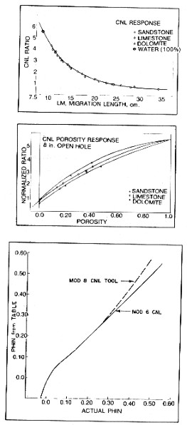 The upper
graph at right
shows the relationship between near and far detector thermal
neutron count rate
ratio versus porosity for the three primary minerals, the data
again being made in laboratory formations. The middle graph shows
the same ratio data plotted against calculated migration length
- Lm. The fit is excellent and even takes in the water point.
The upper
graph at right
shows the relationship between near and far detector thermal
neutron count rate
ratio versus porosity for the three primary minerals, the data
again being made in laboratory formations. The middle graph shows
the same ratio data plotted against calculated migration length
- Lm. The fit is excellent and even takes in the water point.