RESISTIVITY IMAGE LOGS
 

This page describes resistivity image logs profiles, in the order of their appearance over the years. This presentation style provides insights into tool evolution, and a specific tool’s capabilities and limitations. You will find most these tool types in your well files – here’s your chance to learn more about them.

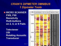
In 1986, the "ultimate" dipmeter was developed by Schlumberger, called the formation microscanner (FMS). Later versions were called formation micro-imager (FMI). There are now similar services available from other suppliers. The tool is generically known as a resistivity image log.

Using an additional 27 electrodes on each of two dipmeter pads of the dipmeter; each pad records 27 microresistivity curves spaced 1/10 inch apart on the borehole surface. Each pad covers a 2.8 inch wide portion of the circumference of the well bore. Several passes over the interval will often provide virtually complete coverage of the rock face.

The resistivity traces are translated into images based on their relative resistivity values, in either black and white or colour. The resistivity data provided by this tool are of very high resolution, in the order of a few millimeters. Thus, a substantially large data array must be handled, and it is an obvious challenge to process and display this information in a way which facilitates its interpretation. This is resolved through a point to point mapping of the resistivity traces into a spatial image, each pixel in the image display having a gray scale or colour value associated with a particular resistivity level. Subsequent interpretation benefits from the close relationship between this image and core photography.

The gray scale or colour spectrum can be stretched or squeezed in the computer to enhance certain features, such as porosity, fractures, or shale laminations. Images can be plotted at the same scale as the core photographs for comparison.

It is traditional to show low resistivity (shales and open fractures) as black, shading to white for high resistivity (tight streaks and healed fractures). Porous sands and shaly sands will be grey or a mix of yellow-brown with darker colour suggesting higher resistivity and possibly lower porosity. In rare cases, such as tar sands and oil shale, the colours may be reversed to make hydrocarbon layers black and shales lighter colours.

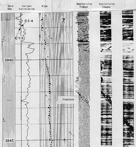
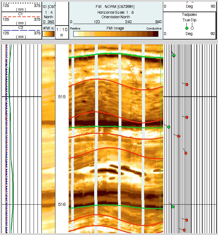
Resistivity image log showing calculates dips, raw curves, and image log from a two pad FMS device.

A resistivity image logging tool with fewer (sixteen) electrodes per pad, but with four or eight imaging pads, is now available, and provides better coverage of the wellbore wall than the two pad version. The electrodes are smaller, allowing for higher vertical resolution, but are spaced to provide the same wall face coverage, about 2.5 inches per pad. In an 8 inch diameter hole, electrode coverage is about 80% and in a 6 inch hole is greater than 100%. This overcomes one of the major complaints about the FMS, namely the number of passes needed to obtain a complete image of the well bore. An example is shown below.

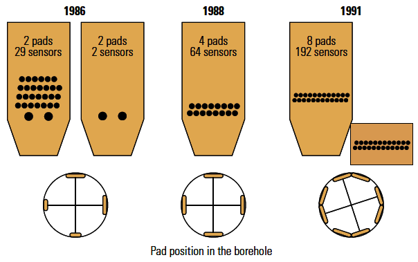
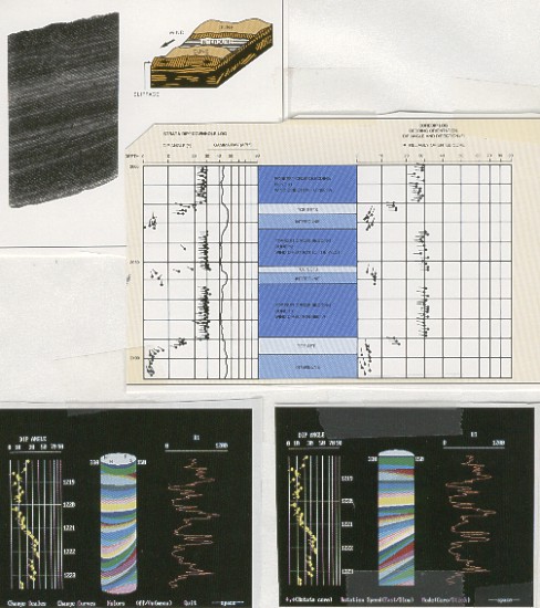
Evolution of the Schlumberger resistivity image log pad design, starting with the original two pad FMS (located on 2 of the 4 pads of the SHDT dipmeter), the four pad FMI (which could be twinned with another tool at 45 degree offset for better borehole coverage), and the eight pad FMI-HD tool (which gives about 98% coverage in an 8" boreho;e).

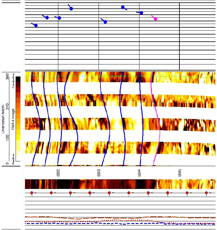
Four pad FMI log in fractured granite reservoir showing computed dip angle and direction. North is at centerline of image.


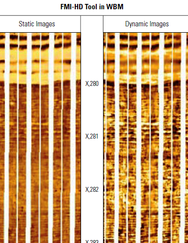
An 8-pad FMI-HD log in a gas shale. Left track is static (fixed colour scale) image. Right track is dynamic image, in which a running average type of colour scaling is used to amplify resistivity contrasts, making easier to see stratigraphic features, faults, and fractures.

The primary use of the tool is definition of bedding plane dips, for identification of irregular features, such as vugs and fractures, for accurate sand counts in thin bedded zones, and for identifying stratigraphic features. If sufficient rock face is imaged, dips can be found by digitizing the bedding planes visible on the microscanner image, or by automatic computation using all valid image traces.

The dips found by FMI dip processing are superior to CSB or LOC dips because a larger number of resistivity traces can be used in the calculation. They can be computed automatically and displayed on the FMS image. In addition, calculated dips can be edited or removed, and new bed boundary correlations picked with a mouse on an interactive CRT image. Thus dips that pass or fail preconceived processing criteria can be deleted or added as the analyst desires. Dip tadpoles can be coded by colour to indicate bedding, cross bedding, fractures, or faults.

RESISTIVITY IMAGE LOG EXAMPLES
 Images courtesy of Schlumberger

Left track is caliper, right track is formation dips. Dip in the cross beds indicate paleocurrents to the WNW direction. This is confirmed by the imbricated shale clasts.
Channel orientation is ESE to WNW


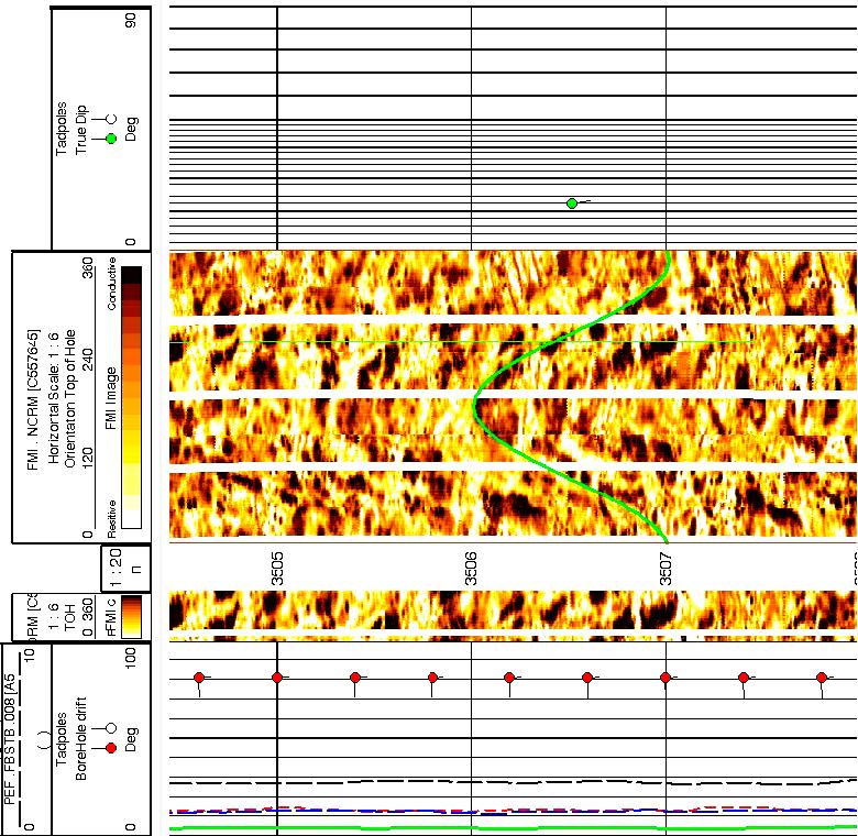
Resistivity images are best dislayed horizontally for horizontal wells-- toe of the well is on the right. Top track is formation or fracture dips, bottom track is borehole deviation. Images illustrate fenestral porosity within a carbonate unit intersected by a horizontal well. Actual well productivity with this type of reservoir is higher than convention open hole logs would indicate.


The slimhole FMS* provides imaging capabilities in boreholes as small a 114mm (4.5 in). This Image reveals a normal fault and fractures in a horizontal well. Fault block downthrown to the N45E direction with 63' dip.






 

Expanded colour scale image of tight streak (light brown) on resistivity image shows detail of porosity laminations - light colour is tight, darker colours are more porous, black is shale.


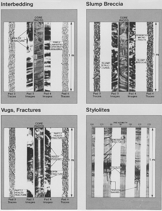
Formation microscanner images in various environments

Formation microscanner images in various environments
 

RESISTIVITY IMAGE LOGS IN OIL-BASE MUD (OBM) SYSTEMS
Material in this section is based on "Imaging - Getting the Picture Downhole" edited by Tony Smithson, Schlumberger Oilfield Review, Sept 2015.

Conventional resistivity image logs require a conductive mud system to operate. In oil based (nonconductive) mud, a knife blade electrode, or "scratcher pad", version of the resistivity image log was available from several suppliers in the later 1980's. The scratcher systems worked reasonably well for bedding dips and sand counts, but could not see fractures very well, because they filled with nonconductive mud.

Schlumberger introduced a new typw of oil-based mud imaging log (OBMI) for use in nonconductive mud systems in 1988. It uses micro induction resistivity measurements instead of the usual electrical resistivity pads. It had 4 pads with 2 rows of 4 electrodes on each pad, operating in the 10 to 20 kiloHertz range. A second tool could be added at 45 degree offset to increase borehole coverage. Resolution vertically and horizontally was about 1 cm, much coarser than the conventional tools (FMS, FMI). It was not very effective in fractures and there were other artifacts that caused shadow events, making the image difficult to interpret in some cases.

The micro-induction technique of older OBM imagers and scratchers of even older dipmeters have been replace by Schlumberger's  Quanta Geo tool. It makes a capacitive measurement at two frequencies in the megaHertz range (instead of the kiloHertz range used in conventional tools) and then derives the best image from the optimal frequency. The tool has 8 pads so the coverage is good compared to other OBM tools. The electrodes are surrounded by guard electrodes that focus current through the mud and mudcale into the formation.

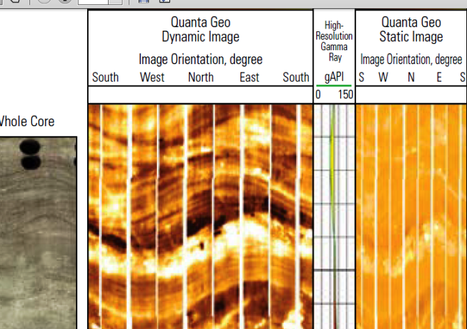
Core image (left), static and dynamic images from Quanta Geo image log

The capacitive measurement allows the processing to determine the amplitude of the current / voltage ratio and the phase shift between the two measurements. The ratio gives the electrical impedance of the rocks. At the frequencies used, the impedance is not directly proportional to resistivity, but the images produced have the same general appearance as conventional image logs. Vertical resolution is 6 mm and horizontal resolution is 3 mm, comparable to the FNI-HD in water based mud. Both open and healed fractures are quite evident on the Quanta Geo output as high resistivity (white) sinusoids. An acoustic image log uld be used to distinguish open from healed.

Fractures (white sinusoids) in oil base mud using Quanta Geo image log. Open fractures cannot be distinguished from healed as both are resistive in OBM.

LOGGING WHILE DRILLING IMAGE LOGS
Measuring resistivity at the drill bit is part of a normal logging while drilling operation. Three resistivity curves sampling different depths of investigation are sent uuole in real-time, along with any other logs in the tool string. Since the tools are rotating while drilling, the deep resistivity scans the entire wellbore as the tool moves slowly down hole. The scanned data is too much to send uphole in real-time and is recorded, then  recovered at the surface when the drill string is tripped for a bit change. Some newer RAB tools can transmit sufficient dats to create an image uphole for near real-time display. Once all the image data is assembled, it can be processed to obtain dip indoemation i a manor similar to wirekine image logs.

Since the density log is also a directionally focused tool that rotates, it too can give an image, although with less contrast than resistivity.

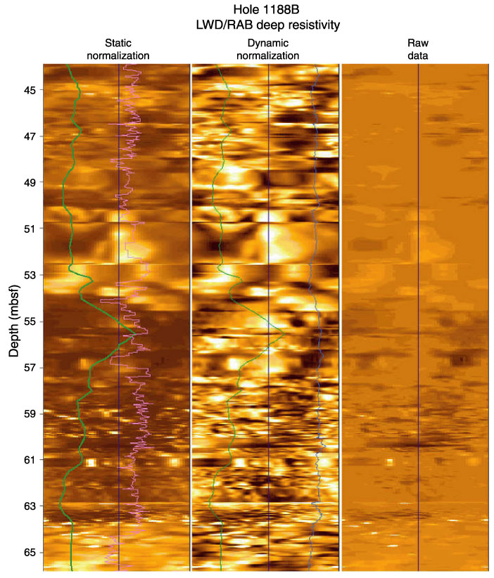
Deep resistivity image from a logging while drilling tool called Resistivity at Bit (RAB). As for all image logs, black represents low resistivity, white is high resistivity. North is at centerline of each image. Since this is a deep resistivity, light colours could mean hydrocarbons or low porosity. Comparison to an open hole FMI or an LWD density image log could resolve the ambiguity.

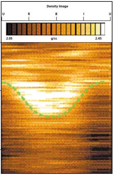
LWD density image log,  black is low density (shale or porous), white is high density (tight). Comparison to RAB
 can identify hydrocarbons: light colour on RAB + dark colour on density image = hydrocarbon. This image is from a
 horizontal well; bottom side of hole is at the centerline of the image.


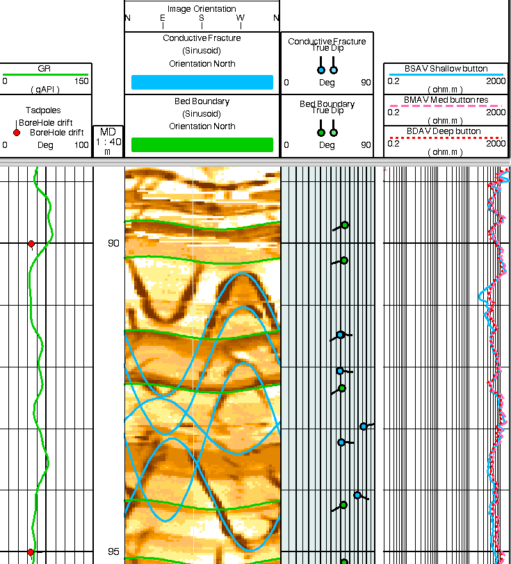
Typical Resistivity-At-Bit (RAB) image log shows gamma ray at left, resistivity image, dip tadpoles, and 3 resistivity curves on the right. This image illustrate open fractures (with blue traces) cross-cutting bedding (in green).

IMAGE LOGS FROM DIPMETERS
Dipmeters and image logs are an essential for assessing structure and stratigraphy of reservoir rocks and for Identification of fracture intensity and fracture porosity. Tool design has improved considerably since its introduction in 1986.

A resistivity image log has about 10 times the spatial resolution of an acoustic image log and 500 times the amplitude resolution, due to the difference in contrast between the resistivity and acoustic impedance ranges measured by the respective tools.

The standard tool works only in conductive mud in open hole, and a specialized tool is available for non-conductive mud. It does not work in cased holes.

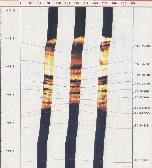
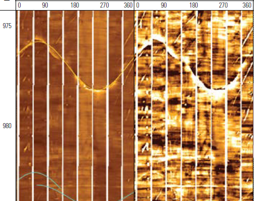
An extension of the stratigraphic high resolution dipmeter (SHDT) processing provides a core-like image of the borehole, using the LOC dip correlations and the measured resistivity curves. The program is called STRATIM (Schlumberger trademark). This image predates the resistivity image log by a few years.

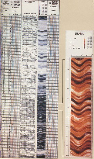
An example is given on the left. The program produces a 360 degree image of the borehole wall by interpolating between the eight resistivity measurements from the eight electrodes on the SHDT pads. Images can be coded in gray scale or colour. Dark gray or dark colour usually represents conductive, often tight shale, beds and light colour resistive, often porous sand, beds. If shales are more resistive than sands (or carbonates), the colour scheme can be reversed to keep shales looking dark.

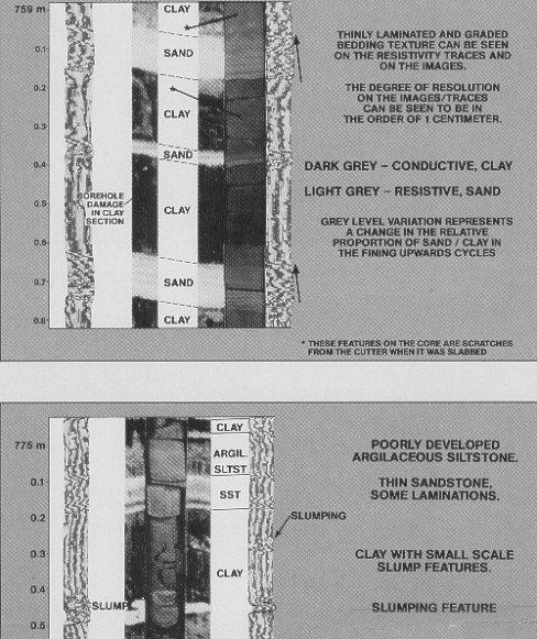
The dipmeter curves are rotated to their true azimuth but are not adjusted to true dip. The dips seen on the image are as they would appear on the surface of a conventional core. The trace of a plane dipping bed forms a sinusoidal curve when the image of the borehole wall is unwrapped and laid flat, as they are in these images. Bed boundaries, dipping beds, slump features, and fractures are easily seen, if present. Images can be enhanced as in Formation Microscanner processing, but processing is cheaper because much less data is manipulated.

A similar program, called DIPVUE is available from Western Atlas, illustrated below. Here the 3-D image can be rotated in real time to view the artificial "core" from any direction. In addition, most core service companies can provide core photographs and dip logs from core data for comparison with log derived borehole images.

The colour convention is to show low resistivity in black and high resistivity in white (or yellow). This makes shale beds black and clean sands white, with shades of grey or brown representing shaly sands. In carbonates, the same rules are used, but white may now mean tight streaks with grey representing porosity. The colour scale can be stretched and squeezed to enhance the image for a particular situation.

Note that a planar, dipping, bedding plane will trace a sine wave on a circumferential image, such as those shown above

DIPVUE image created from dipmeter data

RESISTIVITY IMAGES FROM MODERN LATEROLOGS
Azimuthal resistivity image logs (a form of laterolog) and high resolution laterologs can be displayed as images as well as resistivity curves. Below is a sample of an array induction (AIT) log and an azimuthal resistivity (AIR) log, the latter showing the azimuthal image log presentation.

 
Comparison of array induction log (left) and azimuthal resistivity laterolog (right). Curve complement and presentations vary considerable with age and contractor. The image log on the azimuthal resistivity presentation is "poor man's" resistivity microscanner log, giving a reasonable sand count  regional dip, and some fracture information. A real microscanner image is shown for comparison (left image).

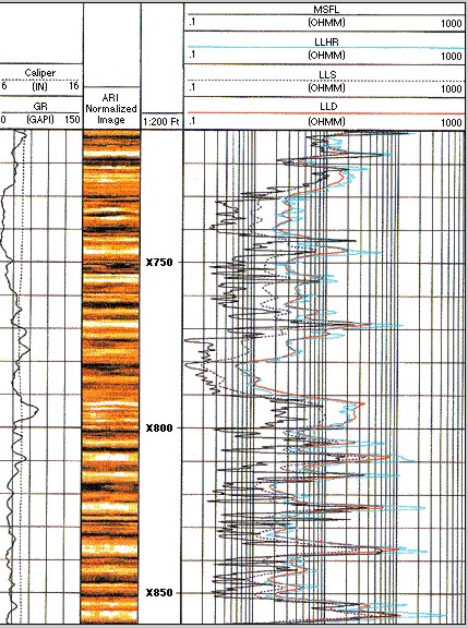
High resolution laterolog showing deep invasion and high resolution image. All curves are focused to
about 8 inches. This tool is not azimuthal so image shows flat-lying beds even when dip is present.fs