The Russians could easily copy the ES. They had confiscated all the Schlumberger equipment and held the crews for several months before releasing them to return home to Paris. The Russians attacked the subject of electrical logging with vigor, developing a multitude of tools with a multitude of spacings and electrode arrangements. The equivalent of the Schlumberger ES Normal curve was called a Potential curve (PZ) and the ES Lateral curve was called the Gradient curve (GZ).
The tool that ran the lateral curve is called a BKZ logging tool. A Spontaneous Potential (PC) curve was recorded with each log run. Only one resistivity curve plus the SP could be recorded on one pass into the well bore, so multiple passes were made to get alternate spacings or electrode configurations. In the early days, this meant that the crew carried a host of different logging tools to the wellsite. Later, a multi-electrode tool was built; jumper wires at the top of the tool allowed the operator to change the electrode configuration without changing tools. The original log with one resistivity curve and the SP was recorded on paper with a stylus or pen recorder, and later on photosensitive paper with a galvanometer. A primitive gamma ray log (GK) and neutron log (NGK), similar to Schlumberger's GNAM and GNT tools, were in evidence by the early 1950's. In the West, two Normals, a Lateral, and an SP could be run simultaneously, using an ingenious electrode switching device called a pulsator. It was a highly sophisticated motorized rotary switch, but very simple in concept; it is surprising that the Russians never duplicate this method of multiplexing several measurements from a single tool.
Later, they developed the equivalent of the Schlumberger Laterolog-7 (BK7) and the Laterolog-3 (BK3), as well as Micrologs and Microlaterologs. In time, they developed an induction log (6F1) similar to a Schlumberger 6FF40, one and two receiver (or two transmitter) sonic logs (AK), a two-detector thermal neutron log (NTK), and a gamma-gamma density log (GGK). Unfortunately for Russia and its neighbours, the more modern technology, easily available in the West, was slow to develop and was not widely distributed. Western Siberia fared the best with numerous sonic and induction logs. The situation has improved considerably in Russia since 1995 when Western service companies made significant progress, but many of the Republics have not done so well. Until recently, the Russian induction log measurement was presented as a conductivity curve, as there was no reciprocal circuit to generate a resistivity curve. No skin effect or shoulder bed corrections were applied at logging time and the maximum resistivity range was 0 - 20 or 0 - 40 ohm-m, depending on tool type. The "K" at the end of each tool abbreviation stands for the Russian spelling of the French word for "well log", "carotage", spelled with a leading "K" (Karotage).
Most of Asia north of Iran and India still use some Russian style
logs, with Western versions on some newer wells, based on specific
joint venture agreements. China has had agreements with Western
service companies for some time, but the old tools can still be used
in more remote regions.
The
Russian to English translation of the core analyses leads to some
confusion. They list both "open" and "effective" porosity,
which have different meanings than in the West. Open porosity means
connected porosity and is equivalent to the porosity from a Boyle's
Law type measurement. In log analysis terms, we call this
"effective" porosity, as it excludes clay bound water. The Russian
style "effective" porosity is actually: Where:
Thus PHIeff is the porosity that could hold hydrocarbons. This has sometimes been called "useful" porosity in the West and is equivalent to the "moveable fluids" in an NMR log analysis model. How SWir is determined for the Russian core analysis report has not been defined in the references available to me. Further confusion is caused by the abbreviations used in Russian reports of all kinds. For example, all laboratory measured rock properties are abbreviated with the letter "K", representing the word "coefficient". Thus Kn is total porosity, Kpo is open porosity, Knp is permeability. Kh represents oil saturation (not horizontal permeability), Kb is water saturation. The subscripts are Russian alphabet, not Roman, so be very careful and read the full words in the report..
Western exploration companies who want to work these areas should acquire and translate the core and sample descriptions. Since it is nearly impossible to calibrate porosity calculations from the unscaled neutron logs without some core control, it is also critical to transcribe all the porosity and permeability data into spreadsheets. Except for translation, these are the same steps we would use to calibrate our work with Western style logs.
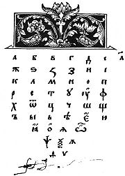
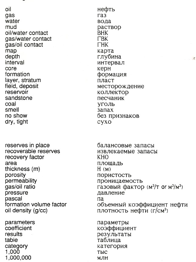
It really helps if you can memorize the pronunciation of the Cyrillic Alphabet, since many technical words and tool mnemonics will sound similar to their English or French counterparts.
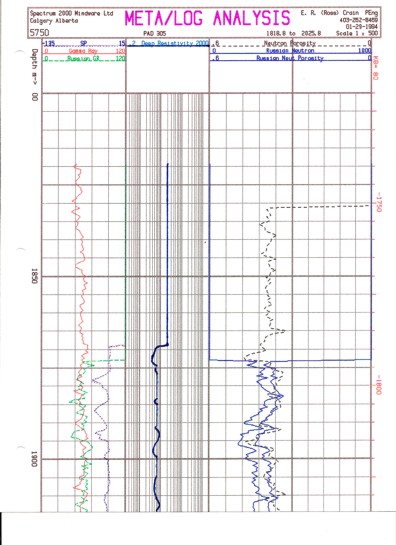
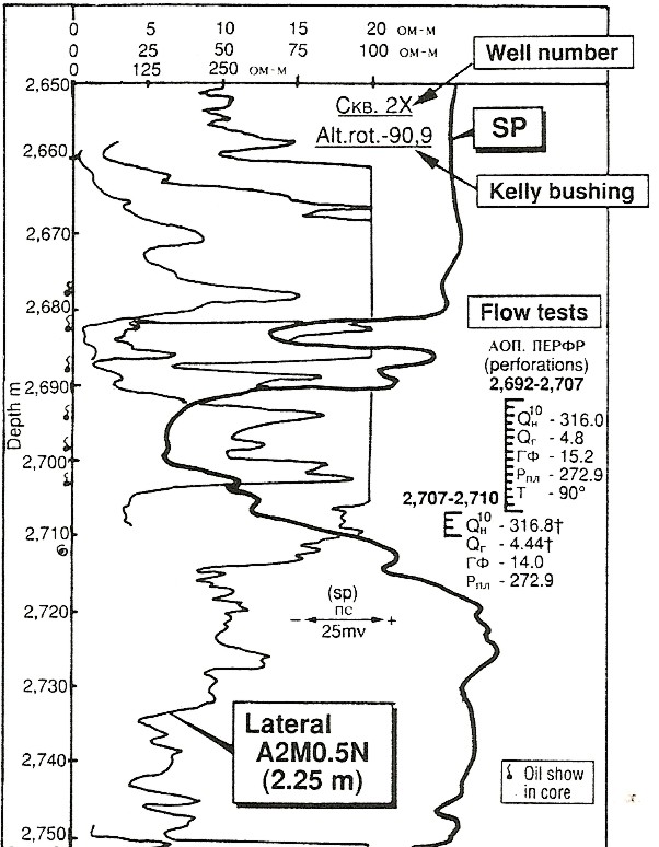
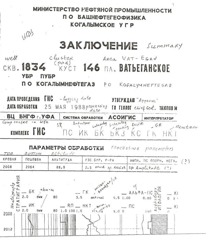
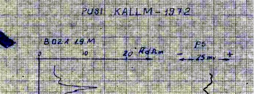
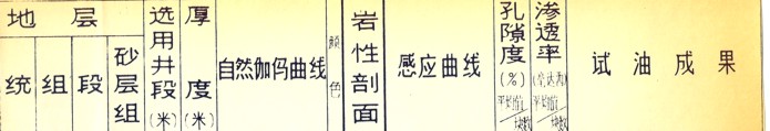
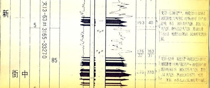
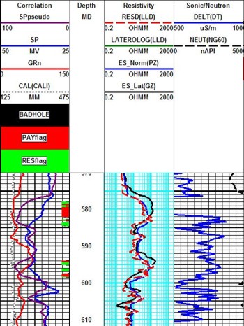
A more typical log heading with curve scales is shown below - hand written data, hand traced curves are the norm. There are no "log tracks", line codes, or curve identification anywhere on the log.
The spacing of the lateral and normal curves is noted at the top of the log near the scale (both handwritten), as for example B2.5A0.5M or M0.75A3B. The letters represent the standard Schlumberger electrode nomenclature and the numbers represents the electrode spacing in meters. For a Normal curve AM is always less than AB. The same electrode arrangement with different spacing can make a lateral curve, for example B0.25A2M, where AM is greater than AB.
Many logs in Russia proper were stamped "KGB Secret" and, at least in the early days after 1991, were filed in different government agencies by log type. The oil production operator had the resistivity logs but a research group elsewhere had the sonic logs. Core and rock data were in a third location with no communication between them. This is still true in some of the less progressive jurisdictions. Since the fall of the Soviet empire in 1991, Russia and most of the Eastern European and Western Asian republics have opened their oil industry to Western service companies. Schlumberger, Baker Atlas, and Halliburton logs can now be found in many of these formerly "closed" countries. It is essential to compare the Russian style logs to modern Western style logs or modern Russian equivalents, just as it is necessary anywhere else in the world when using "ancient" logs.
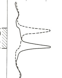
Inverse lateral
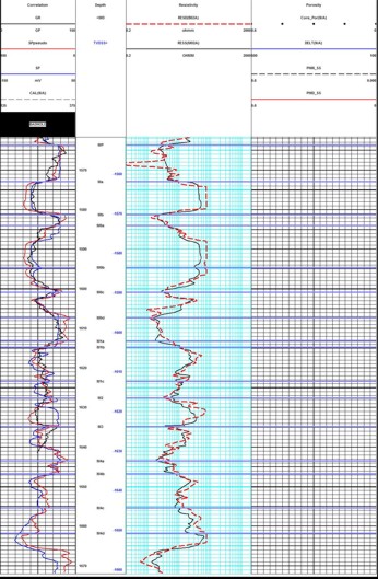
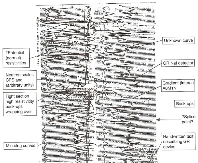
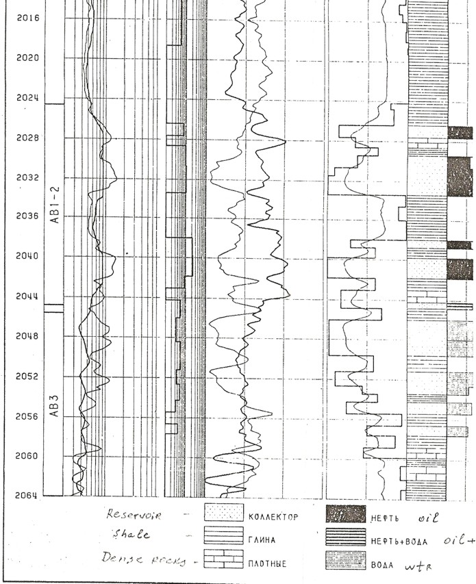
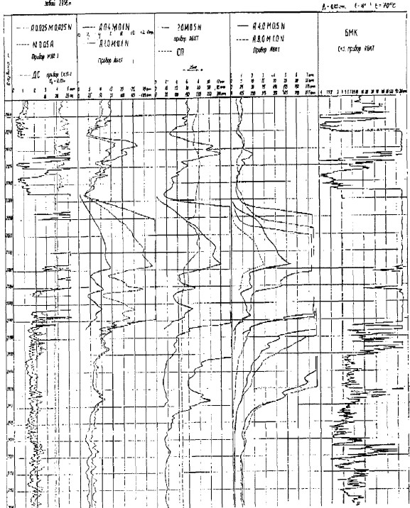
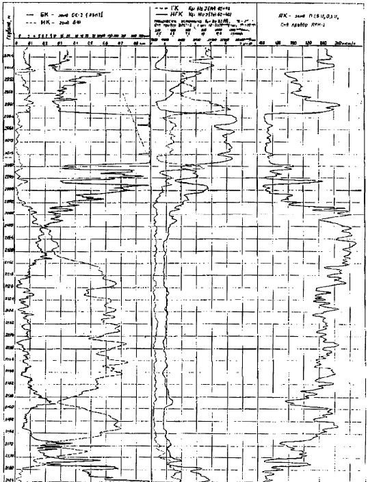
(dotted curve) and original lateral (solid curve) The blind spot is the thickness of the tool spacing, a few to several meters for typical Russian and Western tools. The blind spot shows low resistivity when it ought to show high resistivity. The lateral curve can be used for handpicked data by following special rules. Because the lateral curve has a blind spot over the top or bottom of every resistive zone, it cannot be used in computer aided log analysis unless some special techniques are used. One approach is to pre-process the data with resistivity inversion software. However, even this sophisticated software is a poor solution, as it tends to draw a straight line through the blind zone, which you or I could do faster and cheaper with a red pencil. Another, more practical, solution is to ignore the lateral data in the blind spot by using appropriate logic in the analysis script, and use a different technique such as Buckles number in these intervals. Water zones must be zoned, but otherwise the technique seems to work well. Depth control was abominable and considerable effort is needed to get the various curves on depth with each other. I use the shallow Normal as the depth reference and move all others to match. The GR may be preferred if it has decent character and is not among the missing. Be sure to find out if the blind spot is on top or bottom before moving lateral curves. Below is a sample Russian log illustrating the confusion of overlapping curves that are commonly seen.
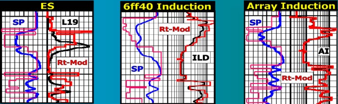
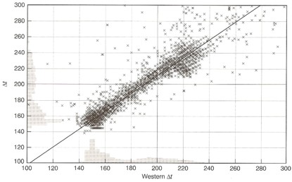
Most FSU wells were drilled with "native mud' so invasion could be quite deep, making SW calculations somewhat erratic. The use of multiple spacing lateral curves was intended to overcome this. The following two illustrations show the changes in resistivity as the tool spacing or tool type is changed. Both images are from "THE ESSENTIALS OF BASIC RUSSIAN WELL LOGS AND ANALYSIS TECHNIQUES" by N. A. Wiltgen, SPWLA 1994.
The general approach used by the Russians was to calculate formation factor from a shallow resistivity log and mud filtrate resistivity, then calculate resistivity index from deep resistivity, after applying all the borehole and invasion corrections to each resistivity curve. This is exactly what petrophysicists in the West did after Archie described his work in 1942.
Porosity was derived from formation factor: Where SXO = 1 - ROS is assumed based on expected oil gravity or from observation of residual oil in cores. Even though this is a well known and formally correct approach, most Russian analysts, and those from the West using older Russian logs, prefer the PHIe = PHIMAX * (1 - Vsh) approach. This is described as the "Porosity from the SP" method in the literature. Westerners generally prefer the GR to the SP for this, but either or both can be used (see next Section below). One reason for this is that RMF was not measured or reported in many cases, and the Russians were fond of experimenting with different mud resistivities in the same borehole, making it difficult to tell what RMF to use in the calculation. PHIMAX came from the "spot" core analysis data.
Saturation is then calculated from Archie's equation: RT, the true (deep) resistivity, came from the laborious manual calculation that corrected for borehole effects, bed thickness, and invasion. In the West, we moved on to use calibrated porosity indicating devices instead of shallow resistivity beginning in 1958, and have continued to improve this technology. Russian technology fell far behind, so Archie's methods based on the ancient ES design persist to this day, because more sophisticated logs are too expensive for most FSU countries, unless they are run by Western joint venture partners. The
Russians did not always admit that the Archie saturation method was
suitable and used more direct but local resistivity transforms. For
example, a curve fit of resistivity to oil volume from cores
(So times PHIe), known as the SOPHI method, works
fine, after you gather enough data. The equations need to be found
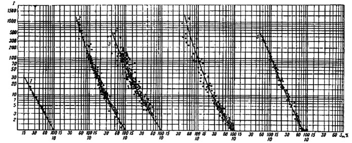
for each local situation. Here is a sample: Below are formation factor and resistivity index plots for a number of Russian oil fields. The slope of a formation factor line is the cementation exponent M and the intercept at 100% porosity is A*RW. The slopes on the resistivity index lines are the saturation exponent N.
The Archie model and its shale corrected versions work well, as long as you do something about editing the asymmetrical kateral resistivity curves.
Water saturation vs resistivity index for five different Russian oil fields, see Wiltgen paper for details.
The Russians
preferred the SP for shale volume, probably because the GR wasn't
run until the well was cased, which would delay analysis. They
actually used an old fashioned formula, still seen rarely in the
West:
Both measured relative to a shale baseline. All
available curves from a recent Russian-style log: If SP is missing, flat, or noisy, we can calculate a
replacement SP. In hydrocarbon bearing sand shale sequences ONLY,: RESD
must be from a long normal or a laterolog (or an induction
log) which are symmetrical curves, and NOT from a lateral curve,
which has a blind spot on top or bottom of pay zones, depending on
electrode arrangement and spacing.
RESS is usually a short normal.
Choosing PHIMAX from a plot of Vsh vs PHIe from offset
wells or core data, high porosity at high Vsh on this plot is from bad
data in rough borehole. In this example, PHIMAX = 0.37.
Neutron counts per second vs porosity for a typical Russian tool
with 60 cm spacing in open hole in limestone. Most neutron logs are
run in casing and in sandstone, so this particular chart will not be
terribly helpful.
Porosity equations for near detector, far detector, and ratio for both thermal and epithermal NTK type tools are available, again for unstated hole conditions.
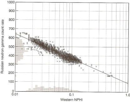
The transform to porosity is usually done with the High-Low semi-logarithmic scaling method. 1. Select a high porosity point on the log, usually a shale, and assign it a porosity based on offset wells with scaled logs or a local compaction curve. This is PHIHI. 2. Pick the count rate on the neutron log at this point - this is CPSHI, even though it is a low numerical value. 3. Choose a low porosity point on the log. Assign this a porosity value, again based on offset scaled porosity logs or core porosity. This is PHILO. Tight lime stringers or anhydrite are best but you need some imagination if there are no truly low porosity streaks. 4. Pick the corresponding count rate on the log. This CPSLO, even though it is a larger number than CPSHI. 5. Plot these points on semi-log graph paper as shown below. Read porosity for any other count rate from the graph.
This graph is
transformed into mathematical terms as follows:
Semi-logarithmic
crossplot of Russian neutron log data in counts per second versus
porosity from a Western neutron porosity log. Similar plots can be
made using core porosity to calibrate Russian neutron logs. Typical accuracy of this type of log is about +/-3% porosity at all porosity levels, about three times worse than a modern neutron log.
Draw vertical line on log at low porosity point (say porosity = 0.05) and another line at high porosity point (usually a shale - say porosity is 0.30). Align scaler between the two lines, setting 0.05 on scaler at low porosity line, and 0.30 on scaler on high porosity line. Skew scaler to obtain good fit. Mark other porosity points on log. Enlarge or reduce scaler in copier to fit smaller or larger logs. High and low porosity points are a matter of good judgment tempered by core or log analysis results from wells with modern logs.
Comparison of
single receiver Russian sonic (Y-axis) with BHCS log, showing higher DTC of
a single receiver tool More recent tools are borehole compensated (BHCS) types, and others have additional receivers approximating an array sonic log. There is no mention in the literature of shear sonic logs. Many Russian sonic logs give unrealistic porosity values, others have chronic cycle skips, mostly to high values.
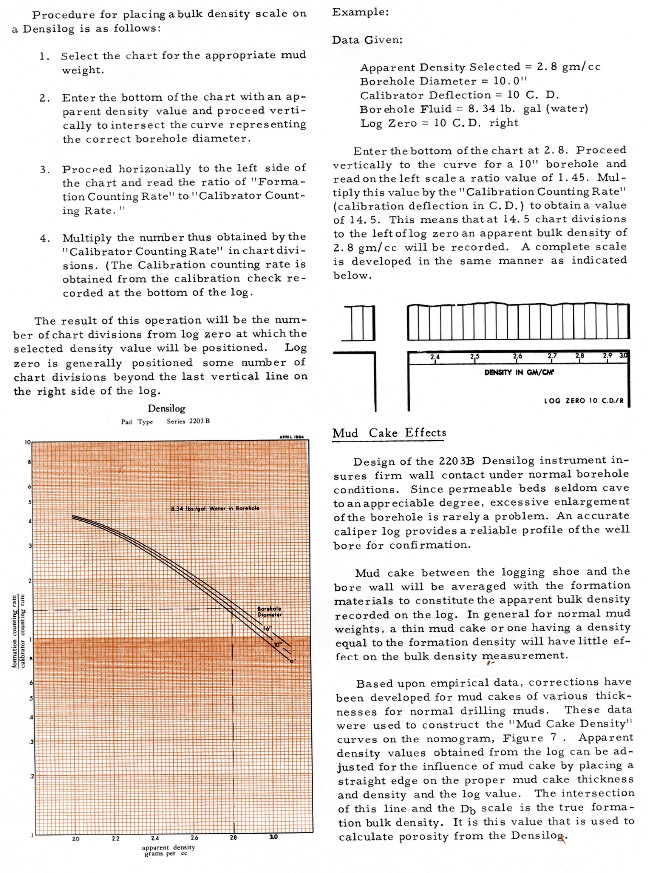
This chart is for
a Schlumberger counts per second 1960's density log, to illustrate
the semi-log relationship that is to be expected for a Russian
density log. The
usual density to porosity transform is used: Most tools were single detector, uncompensated types. These are severely affected by hole size, mud weight, mud cake thickness, source type and strength, source detector spacing, and detector efficiency. The High-Low calibration method compensates for all these problems, but available charts do not. In the earliest versions of these tools, the source strength decayed at the rate of about 1% per week, so count rates definitely need to be normalized on a well by well basis. Similar tools, with better sources, were available in North America in the mid 1960's. I actually ran such logs in slim sulphur-exploration strat holes in the Canadian Arctic Islands in 1969. Newer Russian density tools are dual detector with some degree of borehole compensation, and some are scaled in gm/cc. An alternate to the semi-log High-Low method was used with early neutron and density logs in the West as well as in Russia. This involves "relative count rate excursions" and service company charts of these values versus the desired rock property (porosity, density). The problem, of course, is that you need the chart unique to each tool and sufficient patience to do the constructions. Below is the instruction set developed by Lane Wells from their 1964 Technical Bulletin on their Densilog Tool..
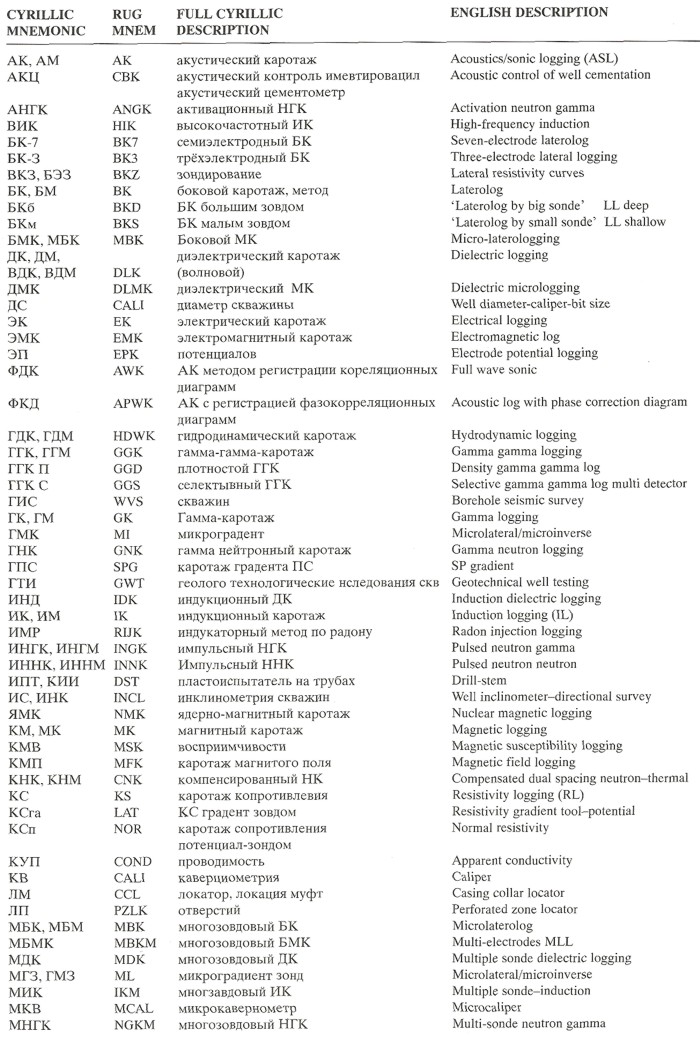
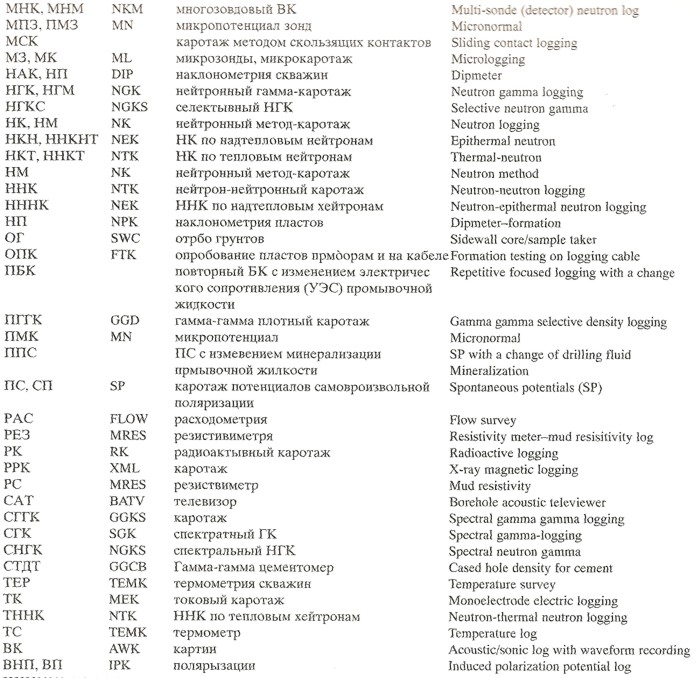
LIST OF TYPICAL RUSSIAN LOGGING TOOL NAMES
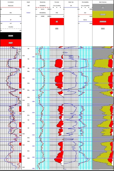
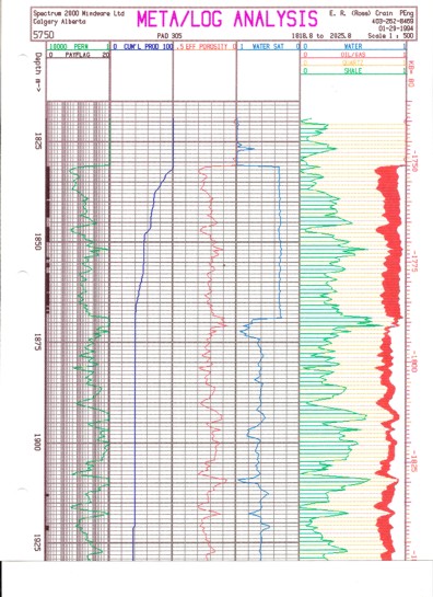
About half the wells had neutron logs. Each was scaled to porosity with the High-Low porosity method. Nearly every well had a gamma ray, so porosity was found from PHIe = PHIMAX * (1 - Vsh). PHIMAX came from the core data. Both porosity curves were compared on a well by well basis and the neutron was discarded where it made no sense. Resistivity was dominated by lateral curves with the blind spot at the top. Standard computer algorithms would have made a water zone at the top of each reservoir layer, so we used Buckle's number to generate Swb = KBUCKL / PHIe / (1 - Vsh). This worked well as there was no need to zone for water. After that, it's common sense and an eye for the ridiculous answer caused by scale or curve choice errors.
Correlation and mapping reserves were more of a political problem,
as our work disagreed dramatically with the Russian version. Obvious
correlations on close spaced wells had been ignored and moved up or
down by as much as 50 meters. We learned in a roundabout way that
oil discovery was done by "quota". If the B zone's incremental
reserves were low, they merely called the A zone the B zone to boost
reserves in the B zone. We flattened all these arbitrary "faults"
and had much more realistic maps. |
|
||
|
Page Views ---- Since 01 Jan 2015
Copyright 2023 by Accessible Petrophysics Ltd. CPH Logo, "CPH", "CPH Gold Member", "CPH Platinum Member", "Crain's Rules", "Meta/Log", "Computer-Ready-Math", "Petro/Fusion Scripts" are Trademarks of the Author |
|||

|
||
| Site Navigation | TOOL PROFILES RUSSIAN STYLE LOGS and ANALYSIS METHODS | Quick Links |
 The
lateral curve on a BKZ tool is not symmetrical and leaves a blind spot at
the top or bottom of a resistive bed (pay zones). This was also true
for ES logs run in the West up to about 1964 when the induction log
finally replaced the last ES. The usual
practice in most parts of the world was to run the electrode
arrangement, called the inverse lateral, that puts the blind spot on
the bottom of the reservoir. Most Russian logs have the blind spot
at the TOP of the reservoir, but either arrangement is possible.
Many wells have both so top and bottom of reservoir layers are
sharply defined. Spacings run from 1 to 12 meters. Typical Western lateral curves
were 5 to 6 meters (15 to 18 feet).
The
lateral curve on a BKZ tool is not symmetrical and leaves a blind spot at
the top or bottom of a resistive bed (pay zones). This was also true
for ES logs run in the West up to about 1964 when the induction log
finally replaced the last ES. The usual
practice in most parts of the world was to run the electrode
arrangement, called the inverse lateral, that puts the blind spot on
the bottom of the reservoir. Most Russian logs have the blind spot
at the TOP of the reservoir, but either arrangement is possible.
Many wells have both so top and bottom of reservoir layers are
sharply defined. Spacings run from 1 to 12 meters. Typical Western lateral curves
were 5 to 6 meters (15 to 18 feet).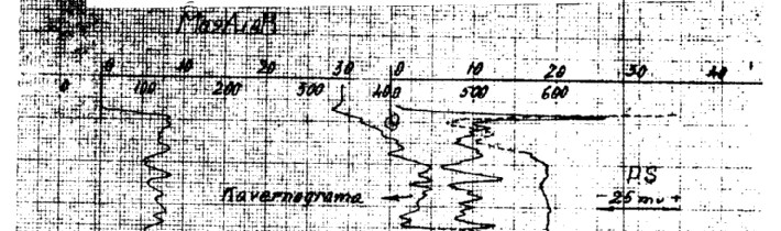
 There
are charts for environmental corrections to Russian logs, similar to
the early departure curve books published in the West during the
1950's. My copy is dated Moscow, 1984 and runs to 180 pages, entirely in
Russian. It was provided by Halliburton around 1992, reproduced from
a Russian Ministry of Oil Industry Geophysical Research Institute
chartbook.
There
are charts for environmental corrections to Russian logs, similar to
the early departure curve books published in the West during the
1950's. My copy is dated Moscow, 1984 and runs to 180 pages, entirely in
Russian. It was provided by Halliburton around 1992, reproduced from
a Russian Ministry of Oil Industry Geophysical Research Institute
chartbook. 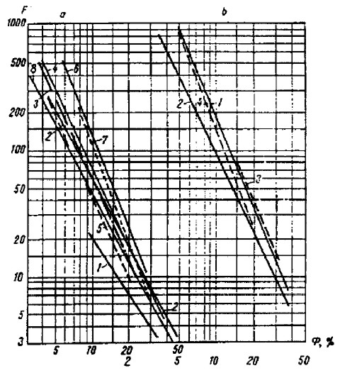
 Gamma ray, SP,
and resistivity curves can be used to calculate shale volume (Vsh) from
the usual equations:
Gamma ray, SP,
and resistivity curves can be used to calculate shale volume (Vsh) from
the usual equations: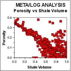 In
FSU wells, there may be no porosity logs of any kind. In
addition, resistivity methods may be ineffective due to lack of
invasion (heavy oil, too much invasion (native mud), or thin bed effects. The maximum porosity
method is quite useful in shaly sands, but may not be helpful in a
carbonate sequence:
In
FSU wells, there may be no porosity logs of any kind. In
addition, resistivity methods may be ineffective due to lack of
invasion (heavy oil, too much invasion (native mud), or thin bed effects. The maximum porosity
method is quite useful in shaly sands, but may not be helpful in a
carbonate sequence: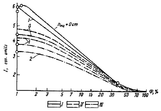 Neutron logs,
usually abbreviated NGK, were the neutron-capture gamma type common to
Schlumberger and others in the 1950's. The detector was very
inefficient and count rates were measured in counts per minute (cpm).
Later tools were scaled in counts per second (cps). Count rate is
inversely proportional to porosity. Charts for specific tools, such
as the one shown at the right, were available to assess porosity.
Neutron logs,
usually abbreviated NGK, were the neutron-capture gamma type common to
Schlumberger and others in the 1950's. The detector was very
inefficient and count rates were measured in counts per minute (cpm).
Later tools were scaled in counts per second (cps). Count rate is
inversely proportional to porosity. Charts for specific tools, such
as the one shown at the right, were available to assess porosity. 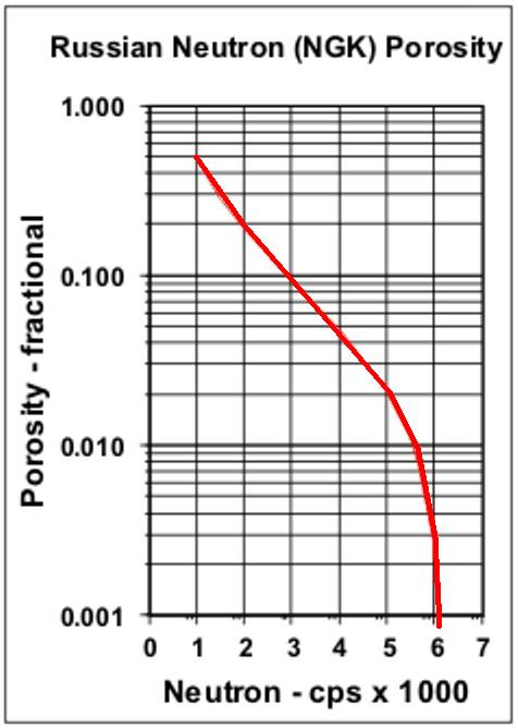 Equations
for neutron porosity were published for various tools, based on a
standard hole size and mud weight, which unfortunately were
unstated. For the neutron capture gamma (NGK) tool with 60 cm
spacing, the equation is:
Equations
for neutron porosity were published for various tools, based on a
standard hole size and mud weight, which unfortunately were
unstated. For the neutron capture gamma (NGK) tool with 60 cm
spacing, the equation is:
 21: INTCPT = PHIHI / (10 ^ (CPSHI * SLOPE))
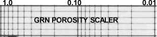
 Russian
sonic logs are in microseconds per meter, mostly uncompensated.
Older tools are single receiver tools that invariably read too high
because of the travel time through the mud. Unfortunately some of
these seem to be still in use.
Russian
sonic logs are in microseconds per meter, mostly uncompensated.
Older tools are single receiver tools that invariably read too high
because of the travel time through the mud. Unfortunately some of
these seem to be still in use. 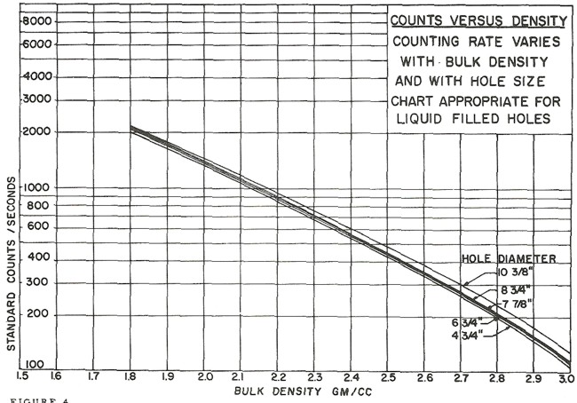 Russian density logs
are mostly recorded in counts per second. You get to work out
the transform to density using a semi-logarithmic High - Low
porosity technique as described above for the neutron log. Here, high
count rate = low density = high porosity. There are published equations for this, but the
parameters required are seldom available, so they are not reproduced
here. Semi-log crossplots of count rate versus core density or core
porosity will resolve this dilemma.
Russian density logs
are mostly recorded in counts per second. You get to work out
the transform to density using a semi-logarithmic High - Low
porosity technique as described above for the neutron log. Here, high
count rate = low density = high porosity. There are published equations for this, but the
parameters required are seldom available, so they are not reproduced
here. Semi-log crossplots of count rate versus core density or core
porosity will resolve this dilemma.