|
 DEPTH PLOT BASICS
Log data depth plots are described by the depth
scale, number of presentation tracks, and the curve names and scales for each
that appear in each track. Logs recorded in the field usually have 3 tracks, one
on the left of the depth values and two on the right, the latter may be combined
into a single wide track. Depth plots that contain computed results, with or
without raw data, can have any number of tracks.
The tables below give details of the common depth scales and curve complement
for a few of the more common log suites. The curve name table shows the
so-called "correlation track" first; it would appear as the left hand track of
almost every depth plot.
A composite plot can merge several log displays into a single plot with any
number of tracks, and may also have tracks with computed petrophysical results.
Customized depth plots are common, but to make life easier for those who have to
use the data, it pays to make the plots as uniform as possible. This means the
curve scale direction, scale values, line colours, line codes, and overall
layout are consistent over time and location.
An excellent low-cost LAS File View and Depth Plot program
is available at
Everett Energy
Software. Follow the link to view a
detailed features list.
PRACTICAL CONSIDERATIONS
Traditional depth plots of well log data are 8.25
inches wide so they can be printed on standard 8.5 inch paper at full size. If
you create a wider plot, printer defaults will shrink both width and length so
it will no longer be at the depth scale you specified. You can still see it full
size on the computer screen but not on a simple printer. Professional software
and wide bed printers overcome this limitation.
For the well log descriptions listed in the tables below, the standard API well log
layout is recommended. It consists of 3 tracks, each 2.5 inches wide, with a
0.75 inch wide depth track between Tracks 1 and 2. See examples in the next
Section. Each track is divided vertically into 10 equal divisions for linear
scales, or into 3 or 4 logarithmic cycles for logarithmic scales.
A log header with log name and well location (and
other useful information) is placed at the top of the log, followed by the curve
names and scale information, centered over the appropriate track. Most log
headers generated by commercial software omits critical information. The header
should include the analyst's name, contact information, and time/date stamp.
There is nothing more frustrating than trying to sort these items out two years
after the plot was made.
For composite plots of raw data or computed results, a 4 track presentation that
fit standard printers is a de facto standard. It consists of a 0.5 inch depth
track on the left, followed by 4 tracks of width 1.875 inches. More width and
more tracks are often seen, but usually at reduced scale when printed, except
for those with expensive wide bed printer/plotters.
An excellent low-cost LAS
File View and Depth Plot program is available at
Everett Energy
Software. Follow the link to view a
detailed features list.
LAS file editing and repair software is available from
KC Petrophysics
(free and commercial versions). Follow the link to view a detailed
features list.
DEFAULT PLOT LAYOUTS
|
STANDARD DEPTH SCALES and GRID LINES |
|
Scale |
Depth # Every |
Grid Lines |
| Ratio |
Units |
Description |
|
4 pt |
2 pt |
1 pt |
| 1:1200 |
English |
1 inch = 100 feet |
100 feet |
200 feet |
100 feet |
20 feet |
| 1:1200 |
Metric |
1 inch = 100 feet |
50 meters |
100 meters |
50 meters |
10 meters |
| 1:600 |
English |
2 inches = 100 feet |
100 feet |
100 feet |
50 feet |
10 feet |
| 1:600 |
Metric |
2 inches = 100 feet |
50 meters |
100 meters |
50 meters |
10 meters |
| 1:480 |
English |
2.5 inches = 100 feet |
100 feet |
100 feet |
50 feet |
10 feet |
| 1:480 |
Metric |
2.5 inches = 100 feet |
50 meters |
100 meters |
50 meters |
10 meters |
| 1:240 |
English |
5 inches = 100 feet |
50 feet |
50 feet |
10 feet |
2 feet |
| 1:240 |
Metric |
5 inches = 100 feet |
25 meters |
25 meters |
10 meters |
1 meter |
| 1:1000 |
English |
1 cm = 100 meters |
100 feet |
200 feet |
100 feet |
20 feet |
| 1:1000 |
Metric |
1 cm = 100 meters |
50 meters |
100 meters |
50 meters |
10 meters |
| 1:500 |
English |
1 cm = 100 meters |
100 feet |
200 feet |
100 feet |
20 feet |
| 1:500 |
Metric |
1 cm = 100 meters |
50 meters |
50 meters |
25 meters |
5 meters |
| 1:200 |
English |
1 cm = 100 meters |
50 feet |
50 feet |
10 feet |
2 feet |
| 1:200 |
Metric |
1 cm = 100 meters |
25 meters |
25 meters |
10 meters |
1 meter |
|
RECOMEMDED DEPTH PLOT LAYOUTS |
|
Curve |
Name |
Left |
Right |
M
or E |
Log / Linear |
Colour |
Width |
Line Code |
| Correlation Track -- All Logs -- Track 1 |
|
|
|
|
|
|
| GR |
Gamma Ray |
0 |
150 |
api |
Linear |
Red |
2 |
Solid |
| SP |
Spontaneous Potential |
-80 |
+20 |
mv |
Linear |
Blue |
2 |
Solid |
|
Metric |
|
|
|
|
|
|
|
|
| CAL |
Caliper |
150 |
375 |
mm |
Linear |
Black |
2 |
Long Dash |
| BITZ |
Bit Size |
150 |
375 |
mm |
Linear |
Black |
1 |
Short Dash |
|
English |
|
|
|
|
|
|
|
|
| CAL |
Caliper |
6 |
16 |
in |
Linear |
Black |
2 |
Long Dash |
| BITZ |
Bit Size |
6 |
16 |
in |
Linear |
Black |
1 |
Short Dash |
| |
|
|
|
|
|
|
|
|
|
Resistivity Logs - All
Types -- Tracks 2 + 3 |
|
|
|
|
|
|
| RESD |
Deep Resistivity |
0.2 |
2000 |
ohm-m |
Log |
Red |
2 |
Long Dash |
| RESM |
Medium Resistivity |
0.2 |
2000 |
ohm-m |
Log |
Blue |
2 |
Short Dash |
| RESS |
Shallow Resistivity |
0.2 |
2000 |
ohm-m |
Log |
Black |
2 |
Solid |
| ** RESxxx |
Optional eg Array RES |
0.2 |
2000 |
ohm-m |
Log |
Blue |
1 |
Dot Dash |
| |
|
|
|
|
|
|
|
|
|
Sonic Logs -- All Types
-- Tracks 2 + 3 |
|
|
|
|
|
|
| DTC |
Compressional Travel Time |
500 |
100 |
ms/m |
Linear |
Blue |
2 |
Solid |
| DTS |
Shear Travel Time |
500 |
100 |
ms/m |
Linear |
Green |
2 |
Solid |
| DTC |
Compressional Travel Time |
140 |
40 |
ms/ft |
Linear |
Blue |
2 |
Solid |
| DTS |
Shear Travel Time |
140 |
40 |
ms/ft |
Linear |
Green |
2 |
Solid |
| ** DTxxx |
Optional eg dipole x-y DT |
-- |
-- |
-- |
Linear |
--- |
2 |
Long Dash |
| |
|
|
|
|
|
|
|
|
|
Alternate for Low
Porosity Rocks |
|
|
|
|
|
|
|
|
Metric |
|
|
|
|
|
|
|
|
| DTC |
Compressional Travel Time |
300 |
100 |
ms/m |
Linear |
Blue |
2 |
Solid |
| DTS |
Shear Travel Time |
300 |
100 |
ms/m |
Linear |
Green |
2 |
Solid |
|
English |
|
|
|
|
|
|
|
|
| DTC |
Compressional Travel Time |
100 |
40 |
ms/ft |
Linear |
Blue |
2 |
Solid |
| DTS |
Shear Travel Time |
100 |
40 |
ms/ft |
Linear |
Green |
2 |
Solid |
| ** DTxxx |
Optional eg dipole x-y DT |
-- |
-- |
-- |
Linear |
--- |
2 |
Lomg Dash |
| |
|
|
|
|
|
|
|
|
|
Density Neutron Logs --
All Types --Tracks 2 + 3 |
|
|
|
|
|
|
| CDN Sand |
|
|
|
|
|
|
|
|
| PHIN_SS |
Neutron Porosity |
0.60 |
0.00 |
fraction |
Linear |
Black |
2 |
Long Dash |
| PHID_SS |
Density Porosity |
0.60 |
0.00 |
fraction |
Linear |
Red |
2 |
Solid |
| PEF |
Photoelectric Effect |
-15 |
+5 |
cu |
Linear |
Purple |
2 |
Dot Long Dash |
| DCOR |
Density Correction |
750 |
-250 |
kg/m3 |
Linear |
Black |
2 |
Short Dash |
| |
|
|
|
|
|
|
|
|
| CDN Carb |
|
|
|
|
|
|
|
|
| PHIM_LS |
Neutron Porosity |
0.45 |
-0.15 |
fraction |
Linear |
Black |
2 |
Long Dash |
| PHID_LS |
Density Porosity |
0.45 |
-0.15 |
fraction |
Linear |
Red |
2 |
Solid |
| PEF |
Photoelectric Effect |
0 |
20 |
cu |
Linear |
Purple |
2 |
Dot Long Dash |
| DCOR |
Density Correction |
250 |
-750 |
kg/m3 |
Linear |
Black |
2 |
Short Dash |
| |
|
|
|
|
|
|
|
|
|
USA Sand |
|
|
|
|
|
|
|
|
| PHIN_SS |
Neutron Porosity |
0.60 |
0.00 |
fraction |
Linear |
Black |
2 |
Long Dash |
| DENS |
Density |
1.65 |
2.65 |
g/cc |
Linear |
Red |
2 |
Solid |
| PEF |
Photoelectric Effect |
-15 |
+5 |
cu |
Linear |
Purple |
2 |
Dot Long Dash |
| DCOR |
Density Correction |
0.75 |
-0.25 |
g/cc |
Linear |
Black |
2 |
Short Dash |
| |
|
|
|
|
|
|
|
|
|
USA Carb |
|
|
|
|
|
|
|
|
| PHIN_LS |
Neutron Porosity |
0.45 |
-0.15 |
fraction |
Linear |
Black |
2 |
Long Dash |
| DENS |
Density |
1.95 |
2.95 |
g/cc |
Linear |
Red |
2 |
Solid |
| PEF |
Photoelectric Effect |
0 |
20 |
cu |
Linear |
Purple |
2 |
Dot Long Dash |
| DCOR |
Density Correction |
0.25 |
-0.75 |
g/cc |
Linear |
Black |
2 |
Short Dash |
| |
|
|
|
|
|
|
|
|
|
Composite Log -- Basic
Raw Data -- 4 Track Grid |
|
|
|
|
|
|
| Correlation |
Track 1 |
|
|
|
|
|
|
|
| Resistivity |
Track 2 |
|
|
|
|
|
|
|
| Sonic |
Track 3 |
|
|
|
|
|
|
|
| Density Neutron |
Track 4 |
|
|
|
|
|
|
|
|
Log curves as defined in each individual log description
|
|
|
|
|
|
|
|
| |
|
|
|
|
|
|
|
|
| |
|
|
|
|
|
|
|
|
| |
|
|
|
|
|
|
|
|
DEFAULT PLOT LAYOUT EXAMPLES
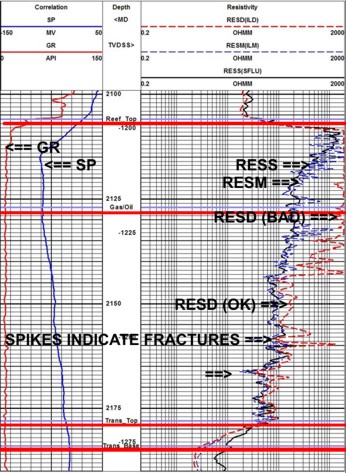
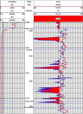
Typical resistivity log (left) and sonic log (right) displayed on
traditional log tracks. Correlation curves in Track 1 to the left of
the depth track and specific log curves in Tracks 2 +3.
Shading on sonic log indicates bad data caused by fractures.
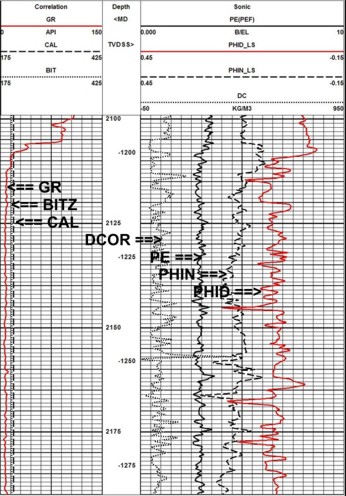
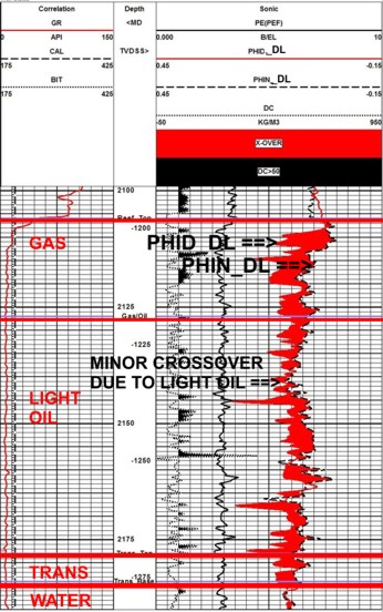
Density neutron PE log on Limestone scale (left) and same log
displayed on Dolomite scale (right). Red shading indicates density
neutron crossover which could indicate light hydrocarbons OR
limestone. PE curve indicates pure dolomite so crossover shows gas
or very light oil.
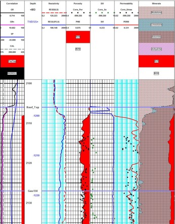
Composite plot in this example combines correlation and resistivity
tracks, with porosity,
saturation, permeability, and lithology results tracks.
|