|
 HEAVY OIL BASICS
Petrophysical analysis of heavy oil reservoirs is quite
straight forward, with one exception. In conventional light
and medium crude oil wells, we expect that a moderate amount
of the original oil in place will move easily to the
borehole and be produced. This is not the case for heavy
oil. The quantity of moveable oil will be quite small and
varies significantly depending on the oil viscosity, gas oil
ratio, drive mechanism, and initial reservoir pressure.
Water floods, miscible floods, and fire floods are used to
encourage oil flow.
Before we discuss the analysis details, lets be sure we have
our definitions straight.
Conventional crude
oil is classified as light, medium, or heavy
according to its measured API gravity.
-
Light crude oil has an API gravity higher
than 31.1 (i.e., less than 870 kg/m3)
- Medium oil
has an API gravity between 22.3 and 31.1 (i.e.,
870 to 920 kg/m3)
-
Heavy crude oil has an API gravity below
22.3 (i.e., 920 to 1000 kg/m3)
Extra heavy crude
oil with API gravity less than 10 ( >1000 kg/m3)
is referred to as
bitumen. Bitumen derived from
oil sands in Alberta has an API gravity of
around 8. It can be diluted with lighter
hydrocarbons to produce
diluted bitumen, which has an API gravity of
less than 22.3 (equivalent to conventional heavy
oil), or further upgraded to an API gravity of 31 to
33 as
synthetic crude (equivalent to conventional
light oil).
Many of the world's heavy oil fields have been in
production for more than 60 years, in places such as
California, Lake Maracaibo, Alberta, Saskatchewan,
China, and former Soviet Union Republics. More are
being expanded and exploited with new technology
today, based on expected rises in oil prices,
erratic as this may be.
LOG ANALYSIS FOR HEAVY OIL WELLS
This page covers the conventional petrophysical analysis
methods for heavy oil, using a volumetric analysis model.
Some analysts prefer a model that uses mass- or
weight-fractions of the components, because it is easier to
calibrate to Dean-Stark core analysis data. The
mass-fraction method is described in the page covering
Bitumen Bearing Oil Sands
and won’t be repeated here.
The usual results from analysis of well logs are shale
volume (Vsh), total and effective porosity (PHIt, PHIe). Lithology (mineralogy), water
saturation (Sw), and permeability (Perm). The first four results tell us
how much oil is present and what kind of rack it is in.
The last item can be used to estimate initial flow rate of
the oil.
In addition, we would like to get a feel for the quantity of
moveable oil in the reservoir. There is a method for doing
this with analysis of the invaded zone water saturation
using a shallow resistivity log. It is not very reliable
because invasion may not be deep enough and the result is
often pessimistic.
In a heavy oil reservoir known to be at or near
initial conditions, core analysis techniques allow us to
obtain estimates of initial water saturation (SWir) and
residual oil saturation (Sro). If these sum to less than
1.00, the balance is moveable oil saturation (Smo):
1: Smo = 1.00 - SWir - Sor
Below are the details of the petrophysical analysis steps
required for a complete evaluation of heavy oil wells.
See
List of Abbreviations
for Nomenclature.
STEP 1: Calculate shale volume.
The most effective method is based on the gamma ray log:
1: Vshg = (GR -
GR0) / (GR100 - GR0)
Adjust gamma ray method for young rocks using the
Clavier equation, if needed:
2: Vshc = 1.7 -
(3.38 - (Vshg + 0.7) ^ 2) ^ 0.5
To account for radioactive sands and volcanics, calculate Vsh from density
neutron crossplot
3:
Vshxnd = (PHIN - PHID) / (PHINSH - PHIDSH)
4: Vshs
= SPR -
SP0) / (SP100 - SP0)
The minimum of these values is selected as shale volume Vsh.
The spontaneous potential (SP) method is not very useful in fresh and brackish
water zones.
STEP 2: Calculate total and effective porosity.
The best method available for modern, simple, log
analysis involves the shale corrected density neutron complex lithology crossplot
model.
Shale correct the density and neutron log data
and calculate total and effective porosity:
5: PHIdc = PHID
– (Vsh * PHIDSH)
6: PHInc = PHIN
– (Vsh * PHINSH)
7: PHIt
= (PHIN + PHID) / 2
8: PHIe
= (PHInc + PHIdc) / 2
This model is quite insensitive to variations in
mineralogy. A gas correction is needed for greater accuracy in gas zones, but
this will not affect the results in heavy oil zones. A graph representing this model
is shown below.
The shaly sand version of the
density neutron crossplot is not recommended because it underestimates porosity
in sands with heavy minerals.
If density or neutron are missing or density is
affected by rough hole conditions, choose a method from the
Handbook Index appropriate for the log curves
available. This includes the use of the PHIMAX method if no porosity logs are
available.
9: PHIt = PHIMAX
10: PHIe = PHIMAX * (1 - Vsh)
Density Neutron Complex Lithology Crossplot
- Oil and Water cases,
or Gas zones with crossover.
STEP 3: Calculate mineralogy.
If the well penetrates a young sand shale sequence, this
step is not usually required as there are few heavy minerals
in the sands. In Lower Cretaceous and older rocks, choose a
method from the Handbook Index
appropriate for the log curves available.
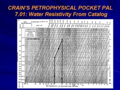
STEP 4: Calculate apparent water
resistivity at formation temperature.
In a relatively clean
nearby water zone, the Archie model using
appropriate electrical properties is sufficient:
11: Rwa@FT = (PHIt ^ M) * RESD / A
Rwa@FT becomes RW@FT in subsequent steps if the
value seems reasonable for your area. Avoid choosing
depleted reservoirs with residual oil for this calculation.
It is useful to also calculate Rwa
at 75F or 25C using Arp's equation, to allow us to
compare log derived values to lab water analysis reports or
water catalogs:
12: Rwa@75F = Rwa@fT * (FT+
6.8) / (75 +
6.8) with temperatures in
Fahrenheit
OR 13: Rwa@25C = Rwa@fT * (FT+ 21.5) / 275 +
21.5) with temperatures in Celsius
If there are no water zones nearby, you will need to use
water catalog data. This will contain RW data at 75F or 25C.
Use equations 12 or 13 to convert measured RW to RW@FT.
RECOMMENDED
PARAMETERS:
for
carbonates A = 1.00
M = 2.00 (Archie Equation as first published)
for sandstone A = 0.62
M = 2.15 (Humble Equation)
A = 0.81 M = 2.00 (Tixier Equation -
simplified version of Humble Equation)
Asquith (1980 page 67) quoted other authors, giving values for A
and M, with N = 2.0, showing the wide range of possible values:
Average sands A = 1.45 M = 1.54
Shaly sands
A = 1.65 M = 1.33
Calcareous sands
A = 1.45 M = 1.70
Carbonates
A = 0.85 M = 2.14
Pliocene sands S.Cal. A = 2.45 M = 1.08
Miocene LA/TX
A = 1.97 M = 1.29
Clean granular
A = 1.00 M = 2.05 - PHIe
META/LOG "RW" Calculate RW
at formation temperature - 5 methods.
Download this spreadsheet:
SPR-07 META/LOG WATER RESISTIVITY (RW) CALCULATOR
Calculate water resistivity (RW),
5 methods,
STEP 5: Calculate water saturation
If the heavy oil sand is relatively clean,
use the Archie equation. If Vsh exceeds about 0.20, use the
Simandoux equation.
Archie Model:
14:
Swa = (A * RW@FT / (PHIe ^ M) / RESD) ^ (1 / N)
Simandoux Model:
15: C = (1 - Vsh) * A * (RW@FT) / (PHIe ^ M)
16: D = C * Vsh / (2 * RSH)
17: E = C / RESD
18: Sws = ((D ^ 2 + E) ^ 0.5 - D) ^ (2 / N)
STEP 6: Calculate permeability and flow
capacity.
In heavy oil zones at or
near initial conditions, we assume SWir = SWa or SWs.
Calculate permeability from Wyllie-Rose equation - results
are in milliDarcies (mD):
19: Perm = CPERM * (PHIe^6) / (SWir^2)
Default for CPRM = 100,000. Adjust to calibrate to core
permeability.
Flow capacity is:
20: Kh = Perm * (BASE - TOP)
Where TOP and BASE are measured depths of top and base of
this aquifer. Note that in a horizontal well, Kh is Perm
times the length of the wellbore exposed to the aquifer.
See
Initial Productivity Estimates to convert Kh to
a flow rate.
META/LOG "PERM" Compare
Permeability Calculated from Various Methods
Download this spreadsheet:
SPR-24 META/LOG PERMEABILITY CALCULATOR
Calculate and compare permeability derived from well
logs,
5 Methods.
STEP 7:
Calculate moveable oil saturation
As
mentioned in the introduction, Smo from core analysis is
preferred:
21: Smo = 1- SQir - Sro
using measured core data values.
From log analysis , we can calculate the invaded zone water
saturation (Sxo). Since invasion is similar to a water
flood, the oil moved away from the wellbore is a good
estimate of moveable oil. The difference between SWa and Sxo
is thus a measure of Smo:
22: Smo = Sxo - SWa
To calculate this step, repeat Step 5 with shallow
resistivity (RESS) instead of deep resistivity (RESD) and
replace RW@FT with RMF@FT. The result will be Sxo.
CAUTION: Because heavy oil is hard to move, invasion is
often very shallow so the shallow resistivity log reads part
of the undisturbed zone. This makes the shallow resistivity
too high, so Sxo is too high and Smo is too low.
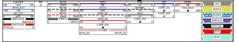
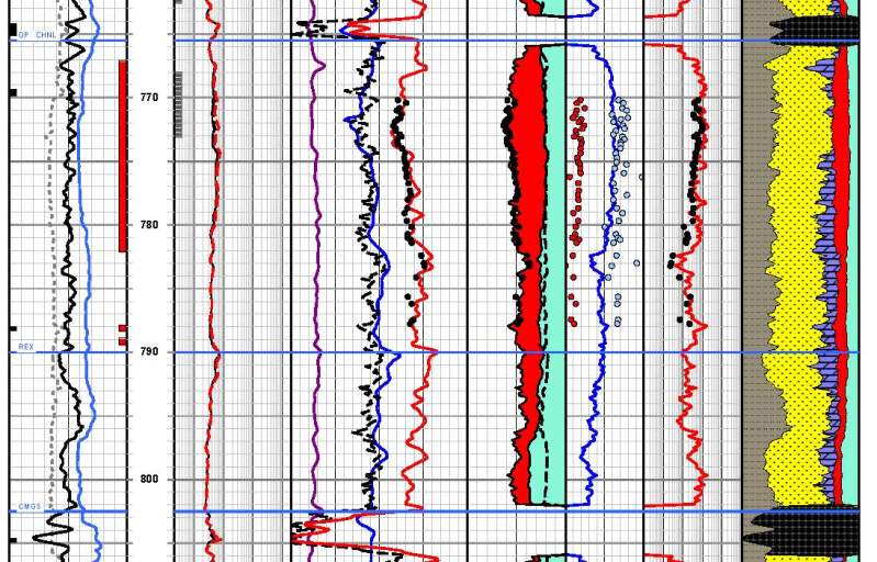
LOG ANALYSIS EXAMPLE IN AQUIFER EVALUATION
These two
examples illustrate the core analysis technique for
assessing moveable oil. Invasion was too shallow for the Sxo
method to work properly. See the captions for details.
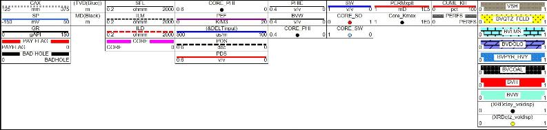
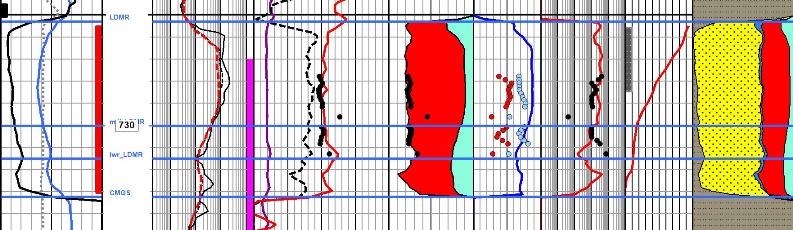
Heavy oil
example with limited moveable oil. Tracks 1 - 3 show raw log
curves. Track 4 shows effective porosity with oil volume
shaded red. Track 5 shows calculated water saturation (blue
line), and core water saturation (blue dots). Notice
excellent match between core and log results. Red dots are
residual oil saturation from core analysis. The distance
between red and blue dots is the moveable oil. Moveable oil
varies from 10 to 30% (1 to 3 grid lines). Permeability in
Track 6 matches core.
Another heavy oil well
with same analysis presentation as the previous example. The
difference is that the distance between red and blue dots is
4 to 5 grid lines, showing considerable moveable oil,
similar to that expected in a more conventional oil well.
This well may have higher gas oil ratio, giving the oil a
lower viscosity and higher mobility.
|