|
 OIL SAND BASICS
Peter Pond called them "tar
sands" in 1778 and in
the early days of the oil business, tar sands were commonly
called tar sands with a little bit of pride. The largest oil
deposit in the world with a 400 year life span could not be
sneered at. In today's politically-correct double-speak, we
now call them "oil sands", not be be confused with
conventional oil sands. So, at the suggestion of a good
friend of mine, this page has been edited to remove the
offensive word wherever possible.
Conventional crude
oil is classified as light, medium, or heavy
according to its measured API gravity.
-
Light crude oil has an API gravity higher
than 31.1 (i.e., less than 870 kg/m3)
- Medium oil
has an API gravity between 22.3 and 31.1 (i.e.,
870 to 920 kg/m3)
-
Heavy crude oil has an API gravity below
22.3 (i.e., 920 to 1000 kg/m3)
Extra heavy crude
oil with API gravity less than 10 ( >1000 kg/m3)
is referred to as
bitumen. Bitumen derived from
oil sands in Alberta has an API gravity of
around 8. It can be diluted with lighter
hydrocarbons to produce
diluted bitumen, which has an API gravity of
less than 22.3 (equivalent to conventional heavy
oil), or further upgraded to an API gravity of 31 to
33 as
synthetic crude (equivalent to conventional
light oil).
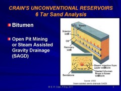
Oil sands (tar sands, bitumen sands) are mined or depleted
by steam assisted gravity drainage (SAGD) or in-situ fire
floods. In all these situations an adequate reservoir
description is needed to assess the economics and progress
of any project.
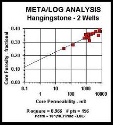
The best oil sands are clean,
medium to coarse grained, unconsolidated sands. However, they may be interbedded with finer, siltier, and shalier sands or overlain by
lower quality reservoir rock. The log analysis needs to describe
these variations, especially laterally continuous barriers to
vertical flow of steam and oil movement.
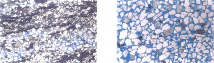
Oil sands at 63 times magnification:
shaly sand (left) with Vsh > 35%,
clean sand (right) with Vsh < 5%.
The
fluid column can be more complicated than conventional
reservoirs. Here are some possibilities:
1. bitumen with or without bottom water
2. top water over bitumen with or without bottom water
3. gas over bitumen with or without bottom water
4. gas over top water over bitumen with or without bottom water
5. any of the above with gas distributed unevenly in the main bitumen
zone.
The oil sands of Alberta appear to be an easy task for a
petrophysicist. After all, the sands are pretty clean, quite porous,
and the fluid properties are reasonably well known. Even a novice
geologist should be able to do it. However, a series of forensic log
analyses over the last 30 years or so suggest that there are some
basic misunderstandings about how oil sand cores are analyzed and
how to calibrate log analysis results to that data.
In each case, the forensic analysis was undertaken at the request of
a client who was unsatisfied with prior work that did not appear to
provide an adequate description of the hydrocarbon potential in an
oil sands reservoir.
 Standard
petrophysical analysis models are used for the volumetric
determination of clay, porosity, water, and oil, and from this a
realistic permeability estimate. Unfortunately, the Dean-Stark core
analysis method, widely used to assess oil sand cores, does not
measure volumes. Instead, the technique measures oil mass, water
mass, and mineral mass. These are converted to mass fraction and
then to calculated porosity and water saturation. Rarely, there may
be some helium porosity and permeability data, but this is difficult
in unconsolidated oil sands. Standard
petrophysical analysis models are used for the volumetric
determination of clay, porosity, water, and oil, and from this a
realistic permeability estimate. Unfortunately, the Dean-Stark core
analysis method, widely used to assess oil sand cores, does not
measure volumes. Instead, the technique measures oil mass, water
mass, and mineral mass. These are converted to mass fraction and
then to calculated porosity and water saturation. Rarely, there may
be some helium porosity and permeability data, but this is difficult
in unconsolidated oil sands.
It is tempting to compare log analysis volumetrics to the Dean-Stark
calculated volumetrics, and adjust log analysis parameters to obtain
a “good match”. The biggest problem is that this form of core
analysis gives a measure of porosity that is sometimes called “total
porosity”, which includes clay bound water. In real life, some of
the clay bound water is not driven off by the Dean-Stark method, so
the core porosity falls somewhere between total and effective
porosity.
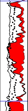
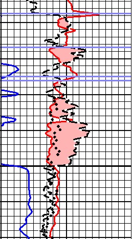
Dean-Stark core analysis (black dots) compared to total porosity
(black curve) and effective porosity (left edge of red shading). 
The calculated water saturation from Dean-Stark also falls somewhere
between total and effective, when some clay is present. Since log
analysis gives effective porosity and saturation, we are comparing
apples to aardvarks. The message is that log analysis cannot be
calibrated directly to the core volumetric data when clay is
present. Virtually all oil sands have some clay content somewhere
in the interval of interest.
But we CAN calibrate to Dean-Stark core data in the mass fraction
domain, by converting the volumetric petrophysical analysis results
to mass fraction. That allows us to compare apples to apples, and
let the aardvarks go about their own business. Oil sand quality is
judged by its oil mass fraction and net pay is determined by an oil
mass fraction cutoff, not porosity and water saturation as in
conventional oil. So oil mass fraction is a mandatory output from a
petrophysical analysis. This approach is also useful for heavy oil
plays (API gravity = 10 -18).
There are additional problems to resolve, as will be discussed
below.
Oil in carbonates is also
extractable with SAGD, fire floods, or solvent floods. Gas is
usually less of an issue because there is less likelihood of
biogenic gas generation, but gas caps may exist in some plays.
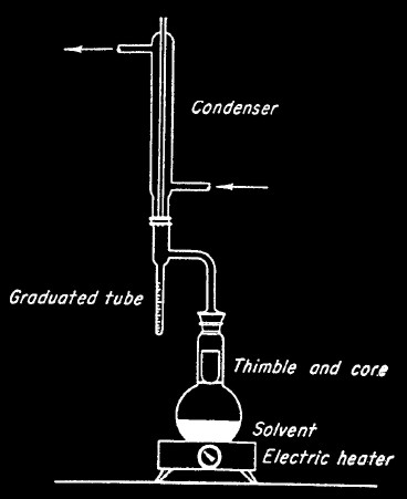 DEAN-STARK CORE ANALYSIS METHOD
This method is used in poorly consolidated rocks such as
oil sands and involves
disaggregating the samples and weighing their constituent
components. Samples are usually frozen or wrapped in plastic to
preserve the contents during transport.
Dean-Stark laboratory apparatus
In the lab, the still
frozen cores are slabbed for photography and description, then
samples are selected and weighed.
Samples are then heated and crumbled to drive off water, and
weighed again. The weight loss gives the water weight. Solvents
are used to remove oil. The sample is weighed again and
the weight loss is the weight of oil. The matrix rock is
separated into clay and mineral components by flotation, dried
and weighed again, giving the weight of clay and weight of the
mineral grains.
1: WTwtr = WTsample - WTheated
2: WToil = WTheated - WTminerals&clay
By dividing each weight by its respective density and
adjusting each result for the total weight of the sample, the
volume fraction of each is obtained. Porosity is the sum of
water plus oil volume fractions Because the bound water in
the clay is driven off by the drying sequences, this porosity is
the total porosity.
3: VOLwtr = WTwtr / DENSwtr / WTsample
4: VOLtar = WTtar / DENStar / WTsample
5: PHIcore = VOLwtr + VOLtar
Assuming clay bound water is driven off by heating and drying,
then PHIcore equals total porosity. From comparison to log
analysis results, it appears that some clay bound water remains
in many cases, so PHIcore lies between total and effective
porosity from log analysis.
Example of Dean-Stark porosity (black dots) showing that it is
less than total porosity from
logs (black curve) due to incomplete drying of clay. Trying to match
log porosity
directly to core may be futile in many cases. Porosity scale is 0.50 to
0.00.
If an oil sand
is consolidated enough to be analyzed by conventional core analysis
instead of Dean -Stark methods (which can handle disaggregated
samples), porosity, saturation , and permeability can be obtained.
No permeability estimate can be made during a Dean-Stark analysis so
permeability data in oil sands projects can be quite sparse.
The table below
shows a comparison of the results from both lab methods.
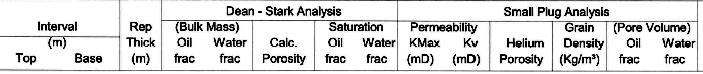
Dean-Stark core analysis in a water
zone in an oil sand play (left side of table) contrasted with
conventional helium porosity analysis .
OIL MASS FROM CORE LISTINGS
If not provided on the core listing, the equivalent value of
oil mass from core analysis
is derived from porosity, oil saturation, and an assumed oil
density:
1: Woil = PHIcore * Soil * DENSoil
2: Wwtr = PHIcore * Swtr * DENSwtr
3: Wrock = (1 – PHIcore) * GR_DENScore
Where:
Soil = oil volume relative to pore volume
Swtr = water volume relative to pore volume
PHIcore = volume of water + volume of oil
Woil = oil mass fraction
Wwtr = water mass fraction
Wrockcore = rock mass fraction
|
PHIcore |
Star |
Swtr |
Vol Oil |
Vol Wtr |
GR_ DEN |
WT Oil |
WT Sand |
WT Wtr |
WT Rock |
Oil Mass Wtar |
Wtr Mass Wwtr |
Rock ``Mass Wrock |
|
frac |
frac |
frac |
frac |
frac |
kg/m3 |
|
|
|
|
frac |
frac |
frac |
|
0.306 |
0.301 |
0.699 |
0.092 |
0.214 |
2.650 |
0.092 |
1.839 |
0.212 |
2.143 |
0.043 |
0.099 |
0.858 |
|
0.271 |
0.236 |
0.764 |
0.064 |
0.207 |
2.650 |
0.064 |
1.932 |
0.207 |
2.203 |
0.029 |
0.094 |
0.877 |
|
0.279 |
0.306 |
0.694 |
0.085 |
0.194 |
2.650 |
0.085 |
1.911 |
0.193 |
2.189 |
0.039 |
0.088 |
0.873 |
|
0.244 |
0.304 |
0.696 |
0.074 |
0.170 |
2.650 |
0.074 |
2.003 |
0.168 |
2.246 |
0.033 |
0.075 |
0.892 |
|
0.298 |
0.217 |
0.783 |
0.065 |
0.233 |
2.650 |
0.065 |
1.860 |
0.233 |
2.158 |
0.030 |
0.108 |
0.862 |
|
0.273 |
0.298 |
0.702 |
0.081 |
0.192 |
2.650 |
0.081 |
1.927 |
0.191 |
2.199 |
0.037 |
0.087 |
0.876 |
Table 1
(above): When saturations and porosity are known (blue shading), all
other terms can be calculated. GR_DENS must be measured or assumed and DENSwtr and DENStar are usually assumed to be 1000 kg/m3. Some core
analysis reports do the math for you, some do not.
Since GR_DENScore represents a mixture of quartz and
shale, this value should vary with shale volume. However shale
volume is never reported on core analysis, so the composite grain
density from the rock sample is used. If grain density is
not recorded in the core analysis, we must assume a constant of 2650 kg/m3 or lower.
FLUID VOLUMES FROM CORE LISTINGS
If not provided on the core listing, the equivalent value of
oil
volumes from core analysis
are derived from porosity, oil mass fraction, and an assumed oil
density:
1: Soil = Woil / (PHIcore * DENSoil)
2: Swtr
= Wwtr / (PHIcore * DENSwtr)
OR 2A: Swtr = 1.00 - Soil
Where:
Soil = oil volume relative to pore volume
Swtr = water volume relative to pore volume
PHIcore = volume of water + volume of oil
Woil = oil mass fraction
Wwtr = water mass fraction
|
PHIcore |
Star |
Swtr |
Vol Oil |
Vol Wtr |
GR_ DEN |
WT Oil |
WT Sand |
WT Wtr |
WT Rock |
Oil Mass Wtar |
Wtr Mass Wwtr |
Rock Mass Wrock |
|
frac |
frac |
frac |
frac |
frac |
kg/m3 |
|
|
|
|
frac |
frac |
frac |
|
0.306 |
0.301 |
0.699 |
0.092 |
0.214 |
2.650 |
0.092 |
1.839 |
0.212 |
2.143 |
0.043 |
0.099 |
0.858 |
|
0.271 |
0.236 |
0.764 |
0.064 |
0.207 |
2.650 |
0.064 |
1.932 |
0.207 |
2.203 |
0.029 |
0.094 |
0.877 |
|
0.279 |
0.306 |
0.694 |
0.085 |
0.194 |
2.650 |
0.085 |
1.911 |
0.193 |
2.189 |
0.039 |
0.088 |
0.873 |
|
0.244 |
0.304 |
0.696 |
0.074 |
0.170 |
2.650 |
0.074 |
2.003 |
0.168 |
2.246 |
0.033 |
0.075 |
0.892 |
|
0.298 |
0.217 |
0.783 |
0.065 |
0.233 |
2.650 |
0.065 |
1.860 |
0.233 |
2.158 |
0.030 |
0.108 |
0.862 |
|
0.273 |
0.298 |
0.702 |
0.081 |
0.192 |
2.650 |
0.081 |
1.927 |
0.191 |
2.199 |
0.037 |
0.087 |
0.876 |
Table 2
(above): If oil mass fraction and water mass fraction are known, as
well as core porosity (blue shading), all other terms can be
calculated. Some core analysis reports do the math for you, some do
not.
OIL SAND MATH
Petrophysical analysis of oil sands follows the standard methods
that have been in use for more than 40 years: The math for these
steps is HERE, except where noted in the
test.
Step 1: Load, edit, and depth shift the full log suite, including
resistivity, SP, GR, density, neutron, PE, caliper, and sonic, where
available. If a thorium or uranium corrected GR (CGR) are available,
load these too. Create a Bad Hole Flag if one is needed.
Step 2: Calculate clay volume. Because some uranium may cause spikes
on the GR, use the minimum of the gamma ray and density-neutron
separation methods. This eliminates false “shale” beds that would
otherwise appear to act as baffles to the flow of steam or oil. The
SP is unlikely to be a useful clay indicator due to the high
resistivity of the oil zone.
Step 3: Calculate clay corrected porosity from the complex lithology
density-neutron crossplot model. This model accounts for heavy
minerals if any are present, compensates for small quantities of gas
if present, and reduces statistical variations in the porosity
values. DO NOT USE THE DENSITY POROSITY LOG ALONE. It will read too
low if heavy minerals are present and too high if gas is present.
The statistical variations at high porosity can give a noisy result.
Some oil sands have enough coal or carbonaceous material to look
like a coal bed. Set a coal trigger on the density and neutron and
set porosity to zero when the trigger is turned on. There is nothing
complex about the complex lithology model, so use it. See “Special
Cases” below if there is gas crossover in the oil zone.
Step 4: Calculate clay corrected water saturation from the Simandoux
or dual-water equations. These default to the Archie model in clean
sands but give more oil in shaly sands.
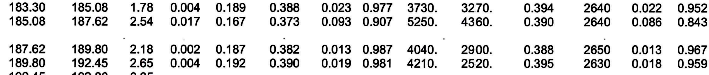
 Step
5: Correlate core porosity and core permeability on a
semi-logarithmic graph, if any data is available. The resulting
equation takes the form Perm = 10^(A * PHIe + B) where A is the
slope and B is the intercept at zero porosity on the graph. Step
5: Correlate core porosity and core permeability on a
semi-logarithmic graph, if any data is available. The resulting
equation takes the form Perm = 10^(A * PHIe + B) where A is the
slope and B is the intercept at zero porosity on the graph.
Step 6: Calculate permeability as a continuous curve versus depth,
using the regression analysis in Step 5.
Steps 1 through 6 cover the conventional volumetric analysis of an
oil sand, but we are not finished yet.
Step 7: Convert log analysis
volumetrics to mass fraction values.
1: WToil = (1 – Sw) * PHIe * DENSHY
2: WTshl = Vsh * DENSSH
3: WTsnd = (1 - Vsh - PHIe) * DENSMA
4: WTwtr = Sw * PHIe * DENSW
5: WTrock = WToil + WTshl + WTsnd + WTwtr
Oil mass fraction:
6: Woil = WToil / WTrock
7: WT%oil = 100 * Woil
Typical densities are DENSMA = 2650, DENSW = DENSHY = 1000, DENSSH
= 2300 kg/m3.
Step 8: A bitumen pay flag is calculated with a log analysis oil
mass fraction cutoff, usually between 0.050 and 0.085 oil mass
fraction. A gas flag should also be shown on the depth plots where
density neutron crossover occurs on the shale corrected log data.
Step 9: Oil in place is calculated from he standard volumetric
equation. However, some operators, especially surface mining
people, work in tonnes of oil in place. This equation is:
1: OILtonnes = SUM (Woil * DENSoil * THICK) * AREA
Thickness is in meters and Area is in square meters.
If the oil equivalent in barrels or cubic meters is needed, the
standard equation can be used:
2: OOIP = KV3 * SUM(PHIe * Soil * THICK) * AREA / Bo
Where:
KV3 = 7758 bbl for English units KV3 = 1.0 m3 for Metric units
AREA = spacing unit or pool area (acres or square meters)
Bo = oil volume factor (unitless)
OOIP = oil in place as bitumen (bbl or m3)
Recovery factor for surface mining operations is very high, maybe
0.98 or better. For SAGD, RF = 0.35 to 0.50 are used. Since we can't
keep the stream away from the shaly sands, recovery will vary with
the average rock quality in a SAGD project.
Water has a very high latent heat, so the volume of water to be
steamed is as important to the economics as the volume of bitumen.
High water saturation is bad news here, just as in conventional oil.
Top water, top gas, and cap rock integrity are also major SAGD
issues. The petrophysical analysis needs to look at the rocks well
beyond the bitumen interval.
GAS EFFECT
AT LOW PRESSURE
 First lets look at the gas problem. If there is no gas crossover,
you can skip this section. The conventional equation for porosity in
a gas sand is: First lets look at the gas problem. If there is no gas crossover,
you can skip this section. The conventional equation for porosity in
a gas sand is:
1: PHIe = ((PHInc^2 + PHIdc^2) / 2) ^ (1 / 2)
This equation is accurate enough for most gas zones,
but in very shallow gas sands, it will underestimate porosity. The
above equation must be replaced by:
2: PHIe = ((PHInc^X + PHIdc^X) / 2) ^ (1 / X)
Where:
X is in the range of 2.0 to 4.0, default = 3.0.
PHIdc and PHInc are shale corrected values of density and neutron
porosity respectively.
Density neutron
crossover in a shallow gas sand with residual oil(shaded
area) and core analysis porosity (dots). The low neutron porosity
indicates little hydrogen content; the effect on the density is much smaller. An X
of 3.0 or higher is needed to calculate effective porosity from logs.
Porosity scale is 0.60 to 0.00
The exponent X is adjusted by trial
and error until a good match to core porosity is obtained.
PARTITIONING GAS and TAR VOLUMES
After
shale volume and porosity have been calculated, water resistivity
can be found in a bottom water zone below the oil, as these rarely
has any residual oil. RW may vary somewhat in the oil sand interval
and this can be adjusted if necessary by comparing calculated oil
mass with core oil mass in non-gassy, relatively shale-free,
intervals. Water saturation is then calculated from a shale
corrected model such as Simandoux.
 Many, but not
all, gas zones related to oil sands have some residual oil.
Hydrocarbon saturation is partitioned between bitumen and gas by the
following method: Many, but not
all, gas zones related to oil sands have some residual oil.
Hydrocarbon saturation is partitioned between bitumen and gas by the
following method:
3: Vwtr =
PHIe * Sw
4: Vhyd = PHIe * (1 – Sw)
5: GasTarRatio = Max(0, Min((1 – OIL_MIN), (PHIDc – PHINc) /
MAX_XOVER))
6: Vgas = GasTarRatio * Vhyd
7: Voil = (1 – GasTarRatio) * Vhyd
Oil weight is calculated from log analysis as follows:
8: WToil = Voil * DENSHY
9: WTshl = Vsh * DENSSH
10: WTsnd = (1 - Vsh -
PHIe) * DENSMA
11: WTwtr =
Vwtr *
DENSW
12: WTrock = WToil +
WTshl + WTsnd + WTwtr
Oil mass fraction:
13: Woil = WToil / WTrock
14:
WT%oil = 100 * Wtar
Where:
OIL_MIN = minimum oil volume in gas zone as seen on core analysis, could be zero.
MAX_XOVER = maximum density neutron crossover in a gas zone (fractional)
Vxxx =
volume fraction of a component
WTxxx = weight of a component (grams or Kg)
Wxxx = mass fraction of a component
WT%xxx = weight percent of a component
 Comparison of
oil mass from log analysis (solid line) with oil mass from
Dean- Comparison of
oil mass from log analysis (solid line) with oil mass from
Dean-
Stark core analysis (dots) Oil mass scale is 0.30 to 0.00. Zone opposite
this
caption is gas with residual oil; above and below are oil with no
gas.
Typical
densities are DENSMA = 2650, DENSW = DENSHY = 1000, DENSSH =
2300 kg/m3. This is the only way to rigourously calculate Oil Mass.
Other equations have been used, such as the one shown below, but are
less accurate, since shale volume is not explicitly enumerated:
99:
Wtar
= ((1.0 - Sw) * Phie * DENStar) / (DENSrna * (1.0 - Phie))
Here, DENSma is a computed result from the log analysis, and is
usually wrong when gas is present. It hides the shale correction
term and individual rock and fluid parameters cannot be adjusted. I
strongly recommend that this "simplified" version be avoided.
It
should be noted that core data is usually derived from a summation
of fluids process, such as Dean-Stark method, so the porosity from
core matches total porosity better than effective porosity. Ditto
water saturation. That's why we use oil mass and not porosity and
saturation to calibrate log analysis to core data.
Oil mass from log analysis is plotted, as shown at
the right, along with oil mass calculated from core analysis data,
on the depth plots to show the match between log analysis and core
data results.
The match between log analysis oil mass, porosity,
and saturation with corresponding core data is usually excellent
except in the very shaly, non-pay, intervals, mostly because the
core data provided ignores shale and its effect on net grain
density. The match in zones with high gas saturation varies in
quality due to the inherent inaccuracy in the gas/oil partitioning
calculation on the log analysis.
META/LOG
"TAR" SPREADSHEET -- Log Analysis in
Oil Sands
This spreadsheet provides a tool for Log Analysis
of Oil Sands, including oil mass, net pay, and
reserves calculations.
SPR-05 META/LOG ESP Advanced Log Analysis Bitumen Sand Metric
and USA
Bitumen Assay -- shale, porosity,
lithology, saturation, permeability, net pay, tar mass
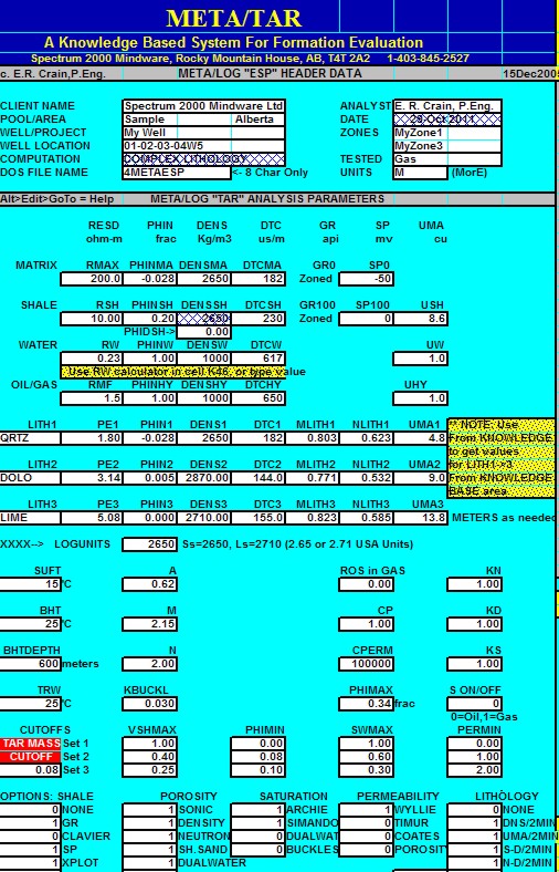
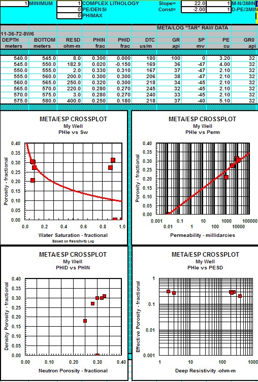
Sample of input data and crossplots for "META/LOG ESP Spreadsheet, used
to analyze oil sand zones.
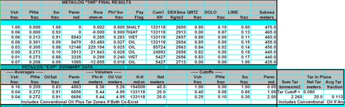
Sample of "META/TAR" net pay summary table.
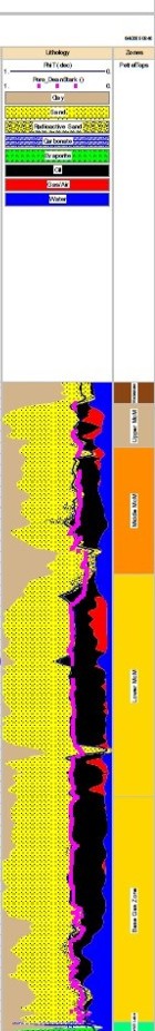
Oil SAND EXAMPLE

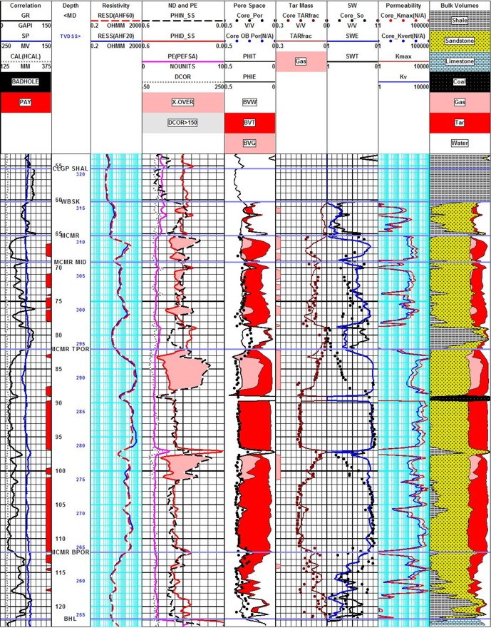
Oil sand analysis with top water, bottom
water, top gas, and mid zone gas. Core and log data match - but oil
mass is the critical measure of success. Core porosity matches total
porosity from logs, due to the nature of the summation of fluids
method used in these unconsolidated sands. Minor coal streaks occur
in this particular area.
Water Satr'n
Statistical |
Fluids
Model |

Fluids
Determinist |

Oil Mass
ic Model |
ALTERNATE MODELS
Comparison of petrophysical methods is often
instructive. In the analysis shown at left, a
probabilistic model (far left) is contrasted with a
deterministic model (right). On the probabilistic model,
oil is black, gas is red, water is blue, and clay bound
water is gray. On the deterministic model, oil is red,
gas is yellow, and water is white. Total porosity from
core (black dots) and total porosity from log analysis
are also shown on the deterministic model.
There are differences in
porosity, especially in the low porosity range,
differences in gas content, and differences in bulk
water volume. Core oil mass (right) was used to
calibrate the deterministic model; the match is
excellent in both gassy and non-gassy oil intervals.
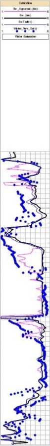
The statistical model
was calibrated by comparing core water saturation to log
analysis saturation (far left). The match is poor in
some oil zones, reasonable in others, and of course is
not a meaningful comparison in gassy zones.
The statistical model
was tweaked several times but was never completely satisfying
because the calibration to core was based on saturation
and not on oil mass.
Oil mass comparison is the only
correct way to match log analysis to core analysis in
oil sand projects.
|
|