Dipmeter computation data are displayed graphically and in tabular
form in many different formats, to facilitate interpretation.
The standard output consists of a raw data plot, arrow plot, and
numerical listings, many of which have been shown earlier in the
discussion of tool and program theory. The balance are optional
at extra cost. They are usually run only after evaluation of the
standard output.
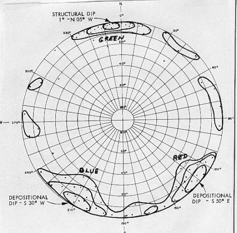
Cylindrical plot in complex cross bedding
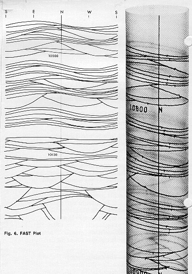
The cylindrical plot is especially useful for locating the position of faults or major unconformities where these are reflected by a change in dip direction or magnitude. The STRATIM and DIPVUE images described earlier offer the same advantages.
The dots will fall into distinctive groupings or patterns, which can be outlined by contour lines. Structural dip is an elongated pattern hugging the outer rim of the plot, possibly extending over a wide range of azimuths. The remaining dips (slope and current patterns) will plot in rough triangles with their apexes pointing toward the center of the plot.
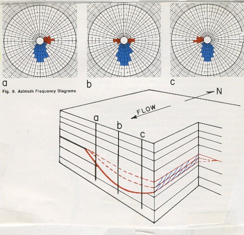
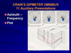
There is no information in the azimuth frequency plot concerning the magnitude of dip. This information must come from other plots. Azimuth frequency diagrams are excellent tools for delineating bars, reefs, channels, and troughs. An illustrative example is shown below, along with a schematic diagram of the channel represented by the frequency plots.
This plot is is called a pattern azimuth frequency plot, because dips belonging to red and blue patterns (to be described later) are preserved and plotted separately. Blue patterns show direction of transport and red patterns show direction to the thicker sand. If plotted in black and white, as is the normal case, the lobes of the diagram are often still identifiable.
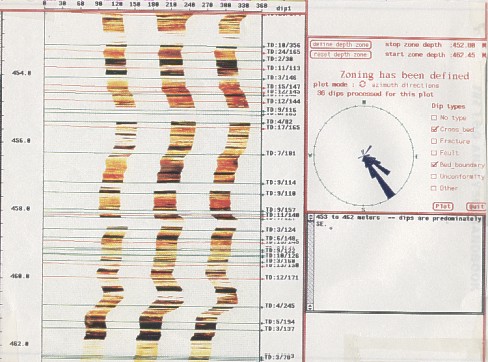
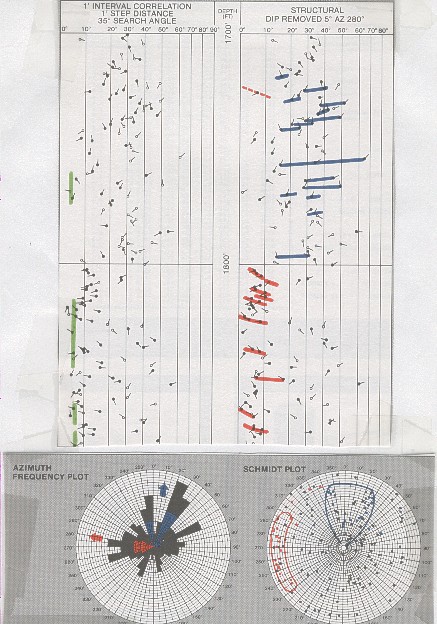
The arrow plot presented to the customer contains azimuth frequency plots generated for each 100 ft. interval or other regular interval as designated by the analyst. These plots are used for general information concerning the direction of dip for each interval of the computed analysis. Additional computer generated azimuth frequency plots can be run over specific zones which have a particular geologic significance. These zones can be the upper and lower boundaries of a formation, the zone between two faults, the zone between a fault and an unconformity or any other breakdown which is indicated by knowledge of the local geology or interpretation of the dipmeter data itself. With the advent of interactive computer programs, decisions on what to plot can be made as processing and analysis take place. using the FMS Image Examiner program.
All
the above plots are available in a hands-on mode when using Schlumberger's
Dipmeter Advisor, and most are available on the Atlas Wireline
DIPVUE program. |
|
||
|
Page Views ---- Since 01 Jan 2015
Copyright 2023 by Accessible Petrophysics Ltd. CPH Logo, "CPH", "CPH Gold Member", "CPH Platinum Member", "Crain's Rules", "Meta/Log", "Computer-Ready-Math", "Petro/Fusion Scripts" are Trademarks of the Author |
|||

|
||
| Site Navigation | DIPMETER PROCESSING AUXILIARY DIPMETER DATA DISPLAYS | Quick Links |
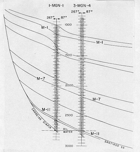
 This
allows the person using the plot to estimate the depth to particular
horizons in the new well. Another use is in correlating formations
from one well to another when both have dipmeter data. The ability
to compute a stick diagram with apparent dip along any defined
azimuth makes it easy to project formation tops from one well
to another. The direction of the stick plot can also be presented
parallel and/or perpendicular to a seismic line and the apparent
dips compared with the dips observed on the seismic line.
This
allows the person using the plot to estimate the depth to particular
horizons in the new well. Another use is in correlating formations
from one well to another when both have dipmeter data. The ability
to compute a stick diagram with apparent dip along any defined
azimuth makes it easy to project formation tops from one well
to another. The direction of the stick plot can also be presented
parallel and/or perpendicular to a seismic line and the apparent
dips compared with the dips observed on the seismic line.