This 3 pronged approach allows the possibility of adapting the interpretation to the specific problem of interest, whether structural, sedimentary, or sand body geometry. SHDT and DUALDIP are Schlumberger trademarks. The three calculation modes described below were extracted from “Applications of the SHDT Stratigraphic High Resolution Dipmeter”, Yves Chauvel et al, Trans SPWLA, 1984.
There is no vertical continuity logic or clustering routine in the MSD computation, and each level is autonomously processed. The clustering is thus replaced by an analysis of the local scattering of the displacements. This method benefits from the ample redundancy available from 28 displacements, while two would be enough to define a dip, reducing the possibility of producing random dips or noise correlations.
With only four side-by-side correlations, the only cross check available is to verify that, for a planar bed, the displacements obtained from opposite pairs of curves (eg. 1-1A and 3-3A) should be equal in value and opposite in sign. This occurs if closure error is zero. If this is the case, any combination of these displacements yields the same dip and any orthogonal pair is used to produce the dip at that depth. If this is not the case, a window is opened around the level under examination, and the vertical continuity of the displacements within the window is checked. The orthogonal pair showing the smoothest continuity within the window is selected for dip computation. Whether a good quality dip (full arrowhead), a low quality dip (open arrowhead), or no dip is output, is a function of the quality of the side-by-side correlations established and of the vertical continuity of the displacements.
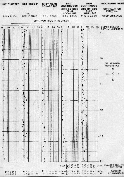
To be retained as a LOC dip, an event has to be recognized on at least 7 of the 8 curves, while the GEODIP logic requires only 3 out of the 4 curves. Thus the LOC dip logic is more demanding than the GEODIP logic, which explains why generally fewer LOC dips are obtained than GEODIP results on comparison runs. The LOC dips are further refined by a cross correlation made on a 12" interval, while GEODIP results are computed directly from the spot events on the curves. This cross correlation involves the eight curves and includes a repetitive best fit and rejection logic as in the MSD computation, with similar criteria for quality coding (full or open arrowhead). A measurement of the planarity is derived from each of the possible dip planes at any level. The retained value corresponds to the surface which best approximates the set of these planes. By convention, a perfectly planar surface has a planarity of 100. Some events are recognized on only some of the dip curves. In this case, the available correlations are traced across the applicable curves, with an optional notation of "F" (Fracture) or of "P/L" (Pebble/Lens) for single pad events or two/three pad events, respectively. These interpretations, however, are not to be considered as certain, but rather as possible. Due to their origin (pad-to-pad correlations), the LOC dips have meaningful lateral significance. If structural dip is present, it will normally be seen by the LOC dips rather than by the CSB dips. Generally the statistical agreement between the LOC and the MSD dips can be expected to be quite good. DUALDIP is the computer program which produces the standard SHDT result presentation. This includes CSB and LOC dips, the eight dip curves, the synthetic resistivity and gamma ray curves, calipers and hole drift data. The depth scale is usually 1/40, and as an option the MSD dips can be added to this output. A sample is shown below.
Structural interpretation is done using the MSD dips. Due to the logic used, namely cross correlation made using long intervals, the MSD dips are the ones likely to represent laterally significant and vertically consistent geological events. For optimum use of the MSD dips, a reduced scale (1/200) plot is normally produced. This plot is also the single SHDT product when no fine scale studies are contemplated. The prime objective of the SHDT tool design is to improve the ability to provide reliable answers to sedimentary interpretation problems. While the rules of interpretation remain essentially the same as in HDT interpretation, there are additional possibilities. Among the information that can be retrieved by visual analysis of the dip curves, reconstructed resistivity, and dip arrows are: - type of lithology (shale, sand, conglomerate) from the shape and likeness of the curves. - fining upwards, coarsening upwards sequences. This is done by analyzing the resistivity variations across the sequence, either with the dip curves themselves or with the synthetic resistivity curve. Other open hole logs, such as the gamma ray (combinable with SHDT), are useful here. Care should be exercised using the resistivity, however, since fluid saturations have to be accounted for when inferring grain size variations from resistivity gradients. - homogeneous bodies (no apparent bedding) as opposed to finely striated, laminated bodies. - parallel vs nonparallel bedding. This is especially important in sandstones, and has found recent applications to the study of turbidites. - correlation lines: some correlations involve the eight resistivity curves, some do not. The most appropriate interpretation (pebble, lens, fracture, other) will be made on the basis of the dip curves (conductive or resistive anomaly, number of pads involved, etc.). - fractures: open fractures will show as isolated conductive spikes which may or may not correlate with similar spikes on other dip curves. Some
of the important uses of the CSB dips are: - determination of the direction of sediment transport, a corollary to the above. This is especially interesting in severe cases of cross bedding, when the only dips produced by long interval correlations generally correspond to those of the individual sedimentary units, seen at their interfaces, and not to the actual current bedding surfaces. - conventional sedimentary interpretation (red, blue patterns, direction of sand body thickening, etc.). All of this can be done on an almost microscopic scale. CSB dips are also very useful, and often better than MSD dips, in high angle apparent dips, when longer correlation intervals are used. LOC dips can be used to study such features as: - nonparallel bedding, for example, when the upper and the lower boundaries of thin beds do not have the same dip. In cases of poor planarity, the event recognition logic will be too tight for a LOC dip to be produced, and the MSD curves may then provide the answer. This is particularly important if this bed is to be found in another well, or when looking for the direction of updip or downdip thickening. - cross bedding: the LOC dips will see the interfaces between the individual sedimentary units, when apparent. This dip may not coincide with the angle and direction of deposition in cross bedded formations (eg. tabular bedding, foreset beds). - turbulence of deposition, when causing non-planarity of bedding. The
MSD dips are normally not used for sedimentary studies, being
the result of an averaging of the dip curve anomalies over the
length of the correlation interval. They are usually presented
on the DUALDIP plots, however, for structural reference. The vertical
(depth) scale used for stratigraphic work makes it difficult to
see structural patterns in the MSD data. |
|
||
|
Page Views ---- Since 01 Jan 2015
Copyright 2023 by Accessible Petrophysics Ltd. CPH Logo, "CPH", "CPH Gold Member", "CPH Platinum Member", "Crain's Rules", "Meta/Log", "Computer-Ready-Math", "Petro/Fusion Scripts" are Trademarks of the Author |
|||

|
||
| Site Navigation | DIPMETER PROCESSING MSD LOC and CSB DIPS | Quick Links |