|
 TiGht Gas ReservoirS-
Deep Basin, Alberta
TiGht Gas ReservoirS-
Deep Basin, Alberta
The Alberta Deep
Basin gas play was “disvovered in 1973, but the presence of
the gas was kmown 10 -15 years earlier because of numerous
blowouts and rig fires that occured during the search for
oil in the area. I arrived at two such fires in a single
week in 1965 with my logging crew, omly to be sent home to
“wait on orders”. So we knew the gas was there, but at 2
cents per mcf and no pipelimes, nobody cared. Ten years
later, Alherta hooked up homes and farms to the gas and we
never looked back.
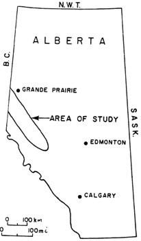 The
material on this page is from a 1981 log evaluation, based
on random wells, undertaken to determine the gas-in-place in
various formations in the Deep Basin area of Alberta. In
addition, comparison of log analysis porosity and water
saturation, core porosity and permeability, and in-situ
(pressure build-up) flow capacity were made in order to find
a relationship between log analysis porosity (or saturation
or both) and well performance. Log to core comparisons were
adequate, but core to in-situ data failed to produce an
acceptable correlation, probably due to fractures not
identified on the core. Thus no method was found, during
this investigation, to predict well performance from log
analysis data alone. The
material on this page is from a 1981 log evaluation, based
on random wells, undertaken to determine the gas-in-place in
various formations in the Deep Basin area of Alberta. In
addition, comparison of log analysis porosity and water
saturation, core porosity and permeability, and in-situ
(pressure build-up) flow capacity were made in order to find
a relationship between log analysis porosity (or saturation
or both) and well performance. Log to core comparisons were
adequate, but core to in-situ data failed to produce an
acceptable correlation, probably due to fractures not
identified on the core. Thus no method was found, during
this investigation, to predict well performance from log
analysis data alone.
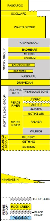 There
are at least 11 productive gas intervals spanning Cretaceous theough
Mississippian wea reservoirs. The gas is trapped by a relative
permeability water block above the gas. See
HERE foe more on thos topic. There
are at least 11 productive gas intervals spanning Cretaceous theough
Mississippian wea reservoirs. The gas is trapped by a relative
permeability water block above the gas. See
HERE foe more on thos topic.
The results were
to be used to help evaluate the resource base in the Deep Basin, and
to provide information needed for deliverability and supply cost
estimates for the area. This paper discusses only the log analysis
methods and results, and does not deal with the supply-cost
estimates which were undertaken by another consulting firm.
To accomplish these objectives, we first computed a Log/Mate
analysis on all prospective zones in 50 wells selected at random
throughout the 200 township area (7200 sq miles). Data from 150
wells (500 zones) in the same area had been studied for other
clients and, with their consent, the core versus log calibration
data and selected results from most of these wells were incorporated
into this study.
Since this data could be from so-called "sweet-spots", the 50 random
wells were thought necessary to remove any bias, and thus prevent
too optimistic a result. We then summarized, for various cutoffs, on
separate data files, the porosity-meters, hydrocarbon meters and net
pay-meters for the 50 random wells and the 150 non-random wells. In
addition, data from 19 specially selected wells were added to
another file, as these wells had extensive pressure build-up data
for correlating log response to productivity.
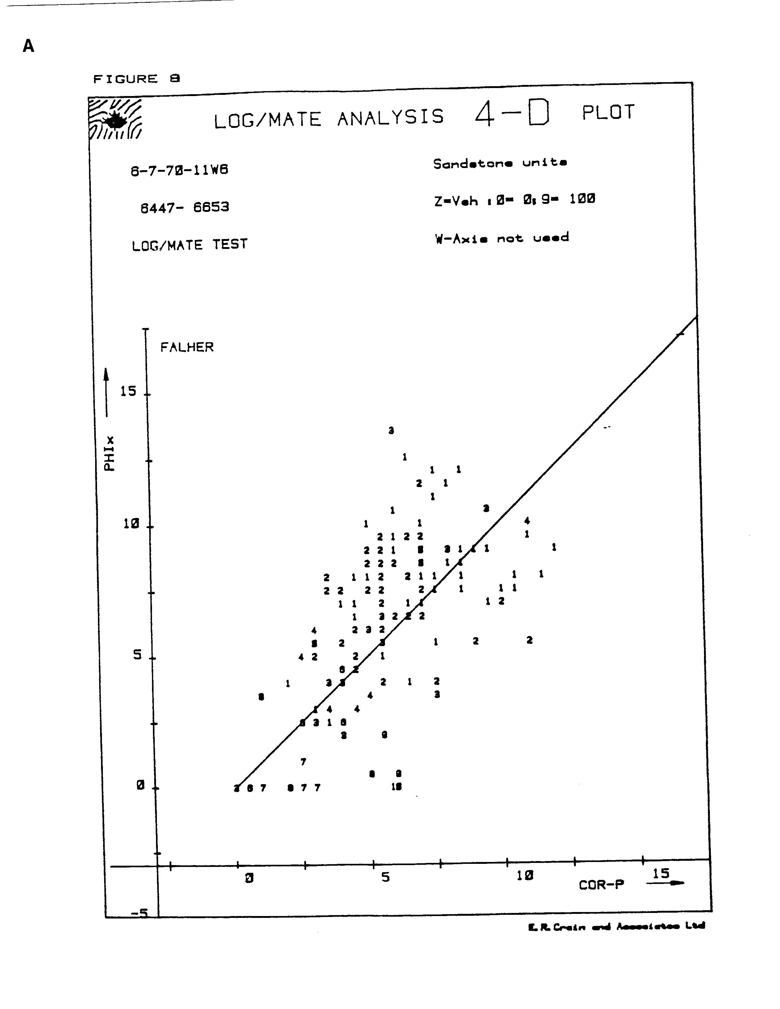
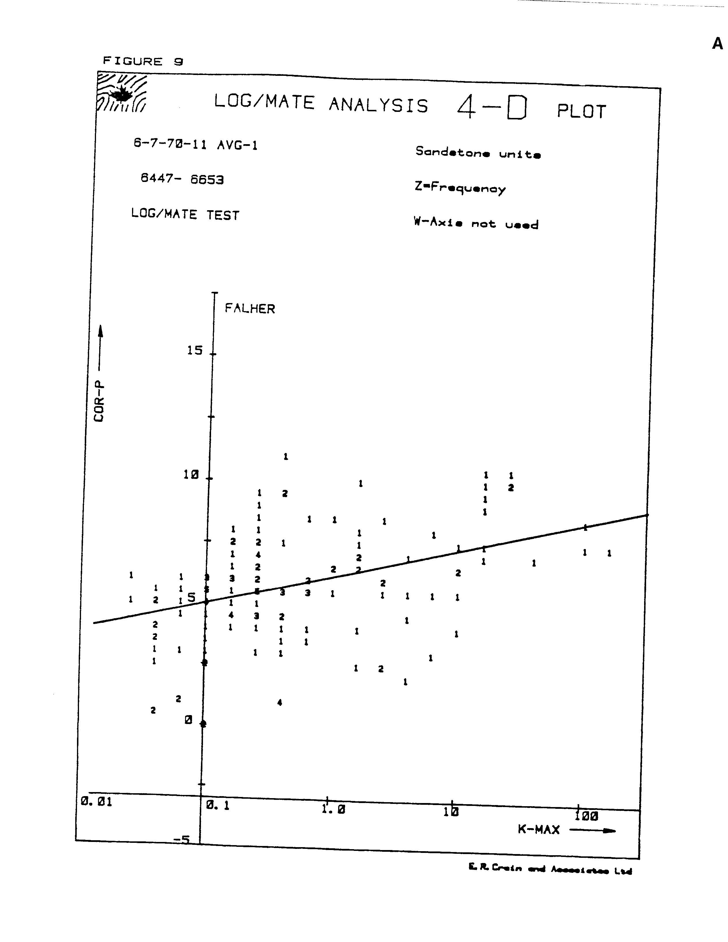
Crossplots of core permeability versus core porosity, and overlays
of core porosity and log analysis porosity were made to demonstrate
the direct relationship between these properties.
Finally, pore volume, hydrocarbon volume and net pay at various
cutoffs were compared to well productivity before and after
hydraulic fracturing. No relationship was found to exist between
these computed log properties and productivity, even though a good
relationship exists between log analysis results and core analysis
data. This likely due to varying amounts of natueal fractures.
This demonstrates that, at least for now, there is an insurmountable
problem in translating gas-in-place figures into economic terms in
tight sands such as these, due mainly to the fact that core
permeability or core derived well productivity does not seem to
correlate with in-situ data from extended pressure build-up data.
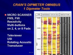
LOG ANALYSIS MODEL and
PARAMETERS
The computation model varied with the data type and quality, and in
order of preference was the following
1. shaly-sand density-neutron crossplot method, where hole
condition permitted and if logs were available,
2. sonic log porosity in bad hole or where density and/or
neutron data was unavailable.(Some wells were done with this method
even when density and neutron log data were available, in order to
meet time deadlines),
3. in zones below the Nordegg,the complex lithology model was
used, which is also a density-neutron crossplot method, with the
sonic log porosity being used in bad hole.
All three of these methods were correct for the presence of shale in
the zone.Shale content was derived from the gamma-ray log response
using a linear interpolation technique.
Various parameters in the interpretation model were varied for each
zone. These reflect changes in the shale, matrix rock and fluid
properties of the zone. The values can be derived in various ways by
comparison with core data. This was done on all wells incorporated
in this study, where core data was available.
Fortunately we have found the values to be quite consistent
throughout the area, provided logs are normalized between wells. A
few wells required shifts to logs to give consistent results. This
was kept to a minimum, and wells were discarded from the study if
the logs were not good enough, or if they required too much editing
and shifting.
The usual parameters for the zones computed in this study are shown
in the table below. These were varied from time to time to account
for perceived changes in tool response between service companies or
for log miscalibration. Standard values of a = 0.62, m = 2.15 and n
= 2.00 were used, since no special core studies were available to
us.
|
TABLE 1:
ANALYSIS PARAMETERS |
|
Zone Name |
Neutron Log
Shale Value
PHINSH% |
Density Log
Shale Value
PHIDSH% |
Matrix
Density
DENSMA
gm/cc
(Kg/m3) |
Sonic Log
Shale Value
DELTSH
usec/ft
(usec/m) |
Sonic Log
Matrix Value
DELTMA
Usec/ft
(usec/m) |
Shale
Resistivity
RSH
ohm-m |
Water
Resistivity
RW@FT
ohm-m |
Formation
Temperature
FT
oF
(oC) |
|
Bad Heart
Cardium
Doe Creek Dunvegan |
30 |
0 to 10
Average 2 |
2.65
(2650) |
81 (265)
to
77 (253) |
55 (182) |
20 |
0.30 |
140 (40) |
|
Paddy Cadotte |
27 |
2 |
2.67 (2670) |
77 (253) |
53 (174) |
20 |
0.20 |
122 (50) |
|
Spirit River Falher |
27 |
2 |
2.69 (2690) |
70 (230) |
51 (167) |
20 |
0.15 |
131 (55) |
|
Bluesky Gething |
27 |
0 |
2.69 (2690) |
70 (230) |
53 (174) |
25 |
0.10 |
149 (65) |
|
Cadomin Nikanassin |
27 |
3 |
2.67 (2670) |
66 (215) |
51 (167) |
20 |
0.07 |
167 (75) |
|
Halfway Doig Charlie Lake |
15 |
-6 |
2.71 (2710) |
60 (197) |
48 (157) |
50 |
0.06 |
176 (80) |
|
Belloy Stoddart Debolt |
10 |
-6 |
2.71 (2710) |
60 (197) |
48 (157) |
50 |
0.05 |
185 (85) |
|
Devonian |
10 |
-6 |
2.71 (2710) |
60 (197) |
44 (144) |
50 |
0.04 |
195 (90) |
Calculations were made with the author's Log/Mate software package
running on HP9835/9845 micro-computers. These systems were sold
commercially beteen 1976 and 1986.
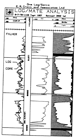
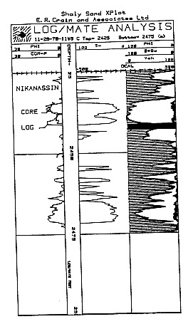
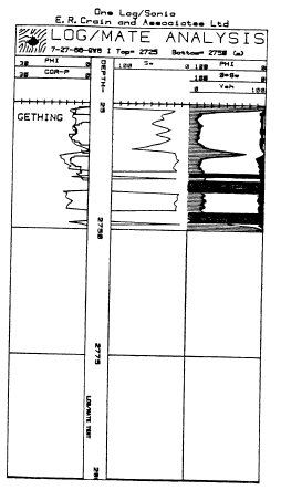
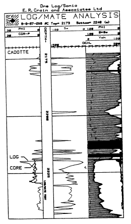
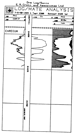
Typical Log/Mate results, alonq with comparisons to core porosity,
are shown below for the Falher, Nikanassin, Gething, Cadotte and
Cardium zones. Note the good match beteeen log and core porosity (in
Track 1). The integration of core data with the log analysis was
vital to the credibility of the project.
To
illustrate the log to core comparison in a different way, we plotted
core porosity versus log porosity crossplots. The example below is
typical for the Falher (same data as Falher depth plot above).
We
have found also that there is a reasonable correlation between core
permeability and core porosity, when plotted on semi-log paper (and
hence a correlation between log analysis porosity and core
permeability). This relationship is shown for a the Falher example
wel. The slope of the best fit line is fairly flat, so small changes
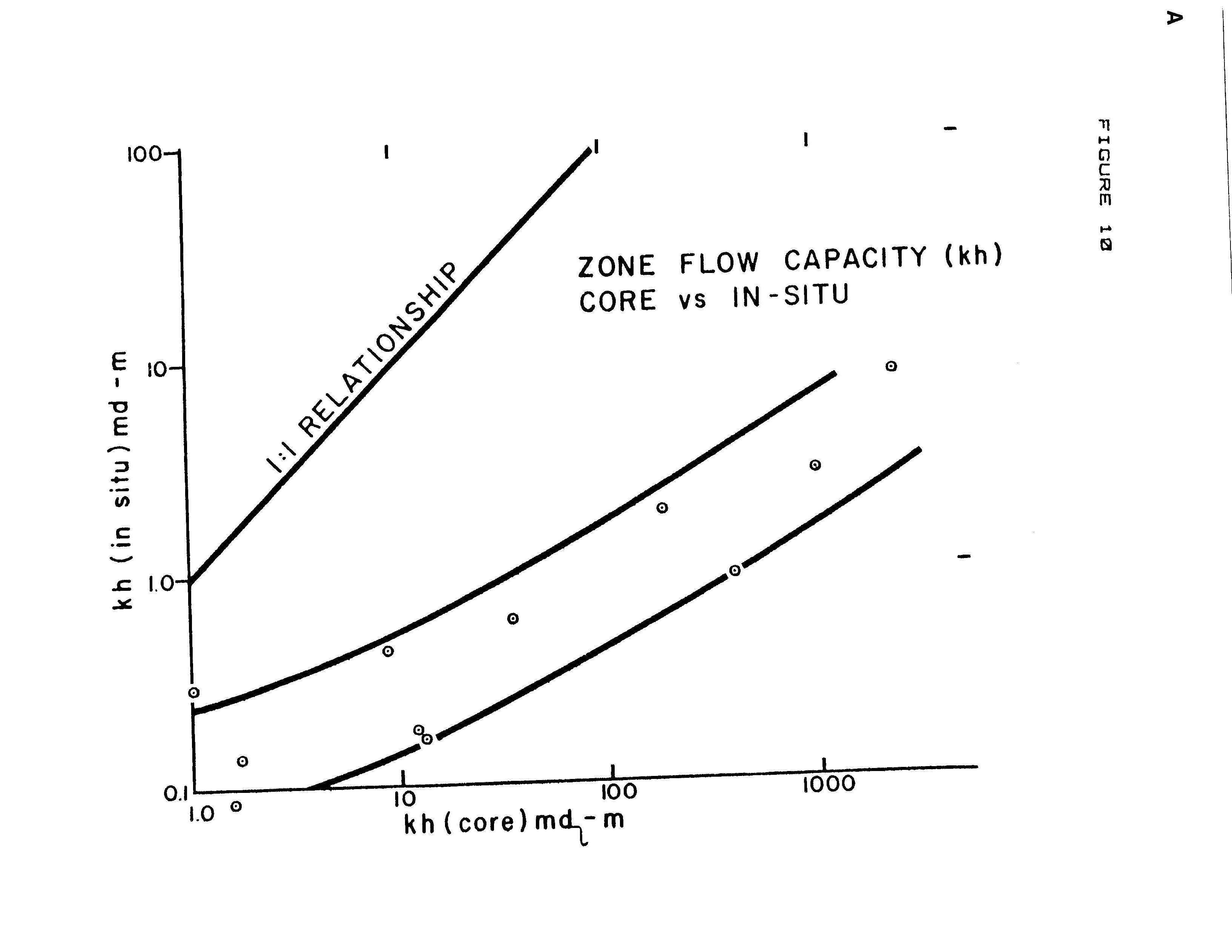
in
Flow capacity (permeability-meters) calculated from core were
compared to insitu build-up test flow capacity. The results for a
few of the more consistent data points is given below, showing a 10
to 1000 times difference
between core and in-situ values.
RESULTS OF THE STUDY
Detailed listings of the pore volume, hydrocarbon volume, and net
pay at various cutoffs were generated for the 41 random wells, for
the 19 special wells, and for the 150 non-random wells. The figures
for the random wells at 5% porosity cutoff are summarized below:
TABLE 2: SUMMARY OF RESULTS
Formation Name
# Zones Avg Net
Pay-Meters
Belly River 1 8.5
Bad Heart 15 2.0
Cardium 35 9.0
Dunvegan 22 8.2
Shaftesbury 1 10.6
Paddy/Cadotte 35 6.1
Spirit River 30 30.1
B1uesky/Gething 31 13.5
Cadomin 17 36.6
Nikanassin 7 23.8
Rock Creek/Nordegg 6 5.9
______________________________
TOTAL 200
AVERAGE PER WELL 4.9 58.8
Data from the 150 non-random wells (possibly biased by
"sweet-spots") and the 19 special wells (definitely biased by
"sweet-spots") produced similar average net pay, average porosity
and average water saturation. This suggests that a large number of
potential gas zones, with thick net pay intervals, and apparently
ubiquitous gas saturation, are present in the Deep Basin of Alberta.
This is no longer news, but some interesting points develop:
1. the log analysis suggests a very high gas-in-place figure
based on the net pay, porosity, and water saturation figures - which
are confirmed by cores,
2. "sweet-spots" of high productivity are not easily seen by log
analysis,
3. much of the gas-in-p1ace is in low porosity rock, which
suggests very low recovery factors at foreseeable wellhead net-back
prices, because of the high cost of delivery of such gas.
|