
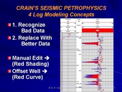
A three well minimum is
recommended for projects. Rarely will the subject well
have all data needed to complete a calibrated
petrophysical analysis. Offset wells should always
be reviewed and used to put together the best data set possible. The accuracy of the
petrophysical model improves with an increased number of wells
reviewed.
|
||||||||||||||||||||||||||||||||||||||||||||
 Logs required are a full suite with resistivity, compressional
and shear sonic, density, neutron, nuclear magnetic, spectral
gamma ray, and caliper logs. LAS (Log ASCII Standard) files
must be reviewed for curve availability. A text editor (Notepad,
Wordpad) can be used to open LAS files to review curve data and
borehole parameters. Measured depth logs should always be
loaded, along with a deviation survey allows reference between
MD, TVD, and TVDSS.
Logs required are a full suite with resistivity, compressional
and shear sonic, density, neutron, nuclear magnetic, spectral
gamma ray, and caliper logs. LAS (Log ASCII Standard) files
must be reviewed for curve availability. A text editor (Notepad,
Wordpad) can be used to open LAS files to review curve data and
borehole parameters. Measured depth logs should always be
loaded, along with a deviation survey allows reference between
MD, TVD, and TVDSS.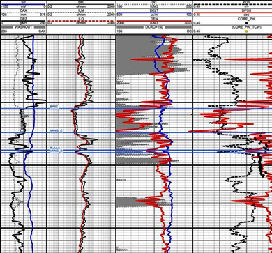
|
Calibrate results
to known lithology from sample descriptions. Adjust trigger
levels to obtain a better match.
Read More about Lithology Triggers
 Step 8: Calculate Total Porosity
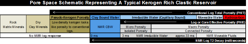
Total
porosity includes clay bound water (CBW). Kerogen will also look like porosity to conventional logs.
Porosity from the neutron
density complex lithology crossplot model is the preferred approach
and is relatively independent of grain density changes.
Other porosity models may also
be used; neutron sonic crossplot
(less sensitive to bad bore hole conditions), density only (very sensitive
to changes in grain density and bore hole conditions), sonic only (very sensitive
to changes in matrix travel time), neutron only (not
recommended, a last resort). NMR total porosity is unaffected by
kerogen and is independent of mineralogy. It is a good alternate
source of total porosity.
Calibrate results
to NMR total porosity or low temperature Dean-Stark core
analysis. Adjust parameters or select alternate porosity model
to obtain a better match.
Read More about Porosity
Step 9: Calculate Effective (Shale
and Kerogen Corrected) Porosity
Effective porosity does not include kerogen effects (in kerogen rich reservoirs) or clay bound water. Shale and kerogen corrected versions of the total porosity models described in the previous section are used to calculate effective porosity.
Calibrate results to NMR effective porosity (3 ms cutoff) or high temperature Dean-Stark core analysis, drives off clay bound water, or conventional helium or Boyle's Law core analysis. Adjust parameters or select alternate porosity model to obtain a better match.
Read More about Porosity
 Step 10: Calculate Lithology
The lithology model must match
the interval being evaluated, and is dependent on available
data. Three mineral models from PE,
neutron and density logs, or from
sonic density and PE logs are best. Two mineral models from sonic
or
density logs may also be useful. Multi-mineral models should be
used with care.
Mineral analysis from logs
is required to reconstruct logs for stimulation design.
Calibrate results
to XRD mineralogy assay, after converting lab data from mass
fraction to volume fraction. Adjust parameters or select
alternate lithology model or alternate mineral mixture to obtain
a better match.
Read More about Lithology
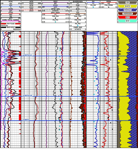
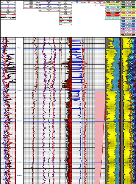
XRD data used to calibrate clay,
quart/feldspar, and carbonate volumes. Doig / Montney interval displaying
elemental capture spectroscopy (ECS) processed mineral volumes,
which were used for lithology model calibration 
Step 11: Calculate Water
Saturation
The modified Simandoux equation
works well for most situations. It accounts for low resistivity
clay content and reduces to the Archie
equation when volume of shale equals zero. This model is better behaved in low
porosity than most other models
dual water models may also
work, but may give silly results when volume shale is high or
porosity is very low.
The tortuosity, cementation and saturation exponents (a, m and
n) are required inputs. In many cases electrical properties must
be varied from world averages to get SW to match lab data.
Recommended values are:
A = 1.0, M = N = 1.5 to 1.8. Lab measurement of electrical
properties is essential.
Water resistivity at reference temperature is required and must be corrected to formation temperature. A deep resistivity log reading and accurate shale and kerogen corrected effective porosity are also required.
Calibrate with core
SW or capillary pressure data. Adjust RW, A, M, N to obtain
better match. Both core SW or capillary pressure data pose problems in
unconventional reservoirs, especially reservoirs with thin
porosity laminations. Common sense may have to
prevail over “facts”.
Read More about Water Saturation
Step 12: Calculate Permeability
Index
The Wylie-Rose equation works
well in low porosity reservoirs. Calibration constant can
range between 100,000 to 150,000 and beyond. Generally assume
that the
calculated SW is also the irreducible SW.
This assumption may not
always be correct.
An exponential equation derived from regression of core permeability against core porosity may also work well. High perm data caused by micro or macro fractures should be eliminated before performing the regression.
Permeability from Wyllie-Rose
Permeability from Regression
Other permeability models are
often used. Any model that can be calibrated to core and uses
log derived properties will do the job. Most models match conventional
core permeability quite well, but will not match permeability
derived from crushed samples using the GRI protocol.
Permeability index from log or core analysis must be
corrected to in-situ conditions before use in flow capacity or
productivity calculations. Log analysis permeability does not
include permeability from micro or macro fractures so flow
capacity from logs may not match KH from pressure transient
analysis. Log perm is usually considered to be matrix
permeability.
Calibrate with
core permeability, excluding fractured samples. Adjust
parameters to obtain a better match.
Read More about Permeability
Step 13: Net Reservoir and Net Pay
Net pay, pore volume, hydrocarbon
pore volume and flow capacity are the final result of most
petrophysical well log analyses. These are called mappable
properties and lead directly to oil and gas in place
calculations.
In many shale gas and some shale
oil plays, typical porosity cutoffs for net reservoir are very
low, 2 or 3% for those with an
optimistic view, 4
or 5% for the pessimistic view.
The water saturation cutoff for
net pay is quite variable. Some unconventional
reservoirs have very little water in the free porosity so the SW
cutoff is not too important. Others have higher apparent
water saturation than might be expected for a productive
reservoir. However, they do produce, so the SW cutoff must be
quite liberal. SW
cutoffs between 50 and 80% are common.
Shale volume cutoffs are usually
quite liberal for unconventional reservoirs, and are usually set
above the 50% mark.
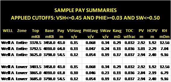
Multiple cutoff sets help
assess the sensitivity to arbitrary choices and gives an indication of the risk or variability in OGIP or OOIP.
Calibration is
not usually possible until years after the field has begun production.
May be possible in flowing wells using flowmeter logs.
Read More about Net Pay and Cutoffs
Step 14: Free Gas or Oil in Place
It is easier to compare zones or wells on the basis of OOIP or OGIP instead of average porosity, net pay, or gross thickness. If area = 640 acres and zone thickness is in feet, then OGIP = Bcf/Section (= Bcf/sq.mile) and OOIP is in barrels per square mile. These units of volume are commonly used to compare zones, wells, or different unconventional plays.
Bg = (Ps * (Tf + KT2)) / (Pf * (Ts + KT2)) * ZF
OGIPfree = KV4 * PHIe * (1 - Sw) * THICK * AREA / Bg
OOIP = KV3 * PHIe * (1 - Sw) * THICK * AREA / Bo
This step is often done by a reservoir engineer on the
evaluation team, based on the petrophysical results developed in
Steps 1 through 13.
Read More about
Gas and Oil in Place.
Step 15: Adsorbed Gas In Place For
Kerogen Rich Reservoirs
TOC is widely used as a guide to
the quality of shale gas plays. Some deep hot shale gas
plays have little adsorbed gas even though they have moderate
TOC content. Using correlations of lab
measured TOC and gas content (Gc), we can use log derived TOC
values to predict Gc. Gc can then be summed over
the interval and converted to adsorbed gas in place, again
measured in Bcf/section to make it easy to compare projects.
Adsorbed gas in place
Gc = KG11 * TOC%
OGIPadsorb = KG6 * Gc * DENS * THICK * AREA
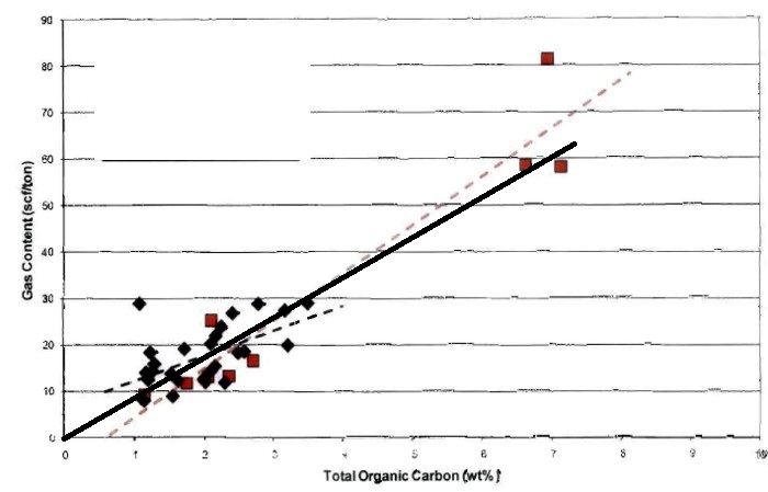
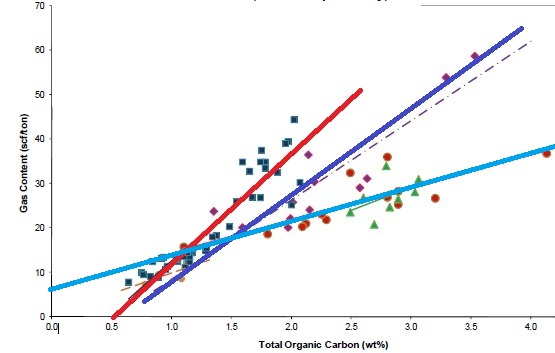
Crossplots of TOC versus Gc for
Tight Gas / Shale Gas examples. Note the large variation in Gc
versus TOC for different rocks, and that the correlations are not
always very strong. These data sets are from core samples; cuttings
give much worse correlations. The fact that some best fit lines do
not pass through the origin suggests systematic errors in
measurement or recovery and preservation techniques, and erroneous
lost gas estimates.
This step is often done by a reservoir engineer on the evaluation team.
Read More about Adsorbed Gas
Step 16: Reconstruct Sonic and
Density Log Curves
For stimulation design
modeling, the logs need to represent a water filled
reservoir conditions. Since logs read the invaded zone,
light hydrocarbons (light oil or gas) make the density log
read too low and the sonic log read too high compared to the
water filled case. Rock mechanical properties are calculated
based on reconstructed logs derived from the petrophysical
analysis. The reconstructed logs eliminate gas effect (if
any) and low quality data caused by rough borehole.
Calibrate
by comparing Vp/Vs ratio (DTS/DTC ratio) with known values for
lithology as computed from petrophysical analysis.
 Read More about
Log Reconstruction
Read More about
Log Reconstruction
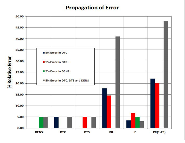
Using
bad sonic data results in erroneous elastic properties ![]()
![]() Effect of porosity and gas on Poisson’s
Ratio. PR will be too low for frac design
purposes unless the water filled case is created by log
reconstruction.
Effect of porosity and gas on Poisson’s
Ratio. PR will be too low for frac design
purposes unless the water filled case is created by log
reconstruction.
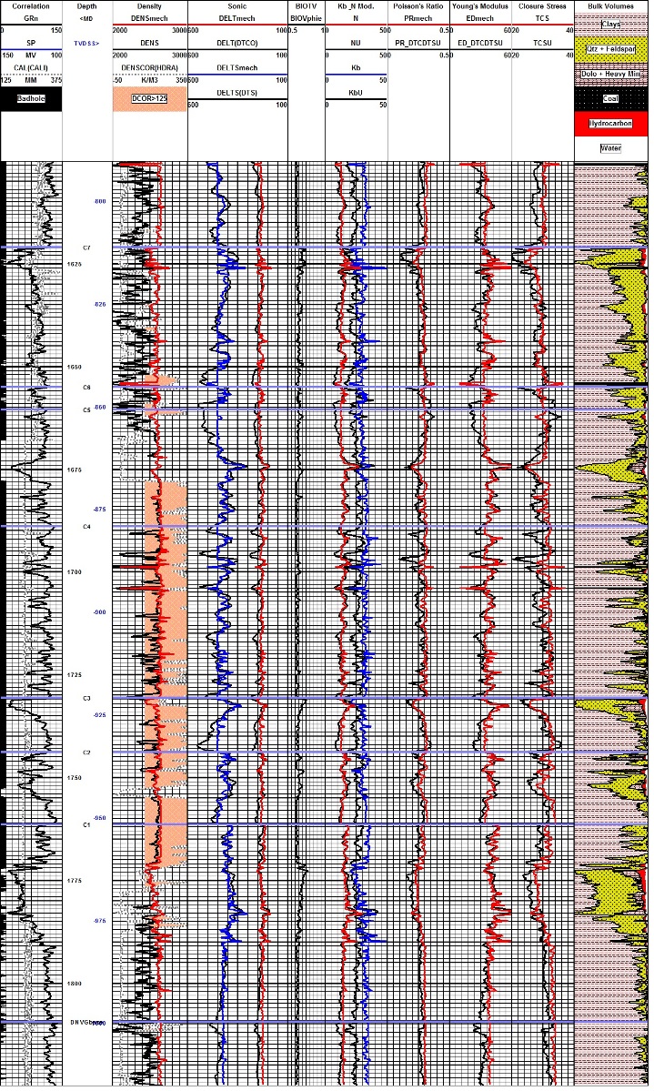
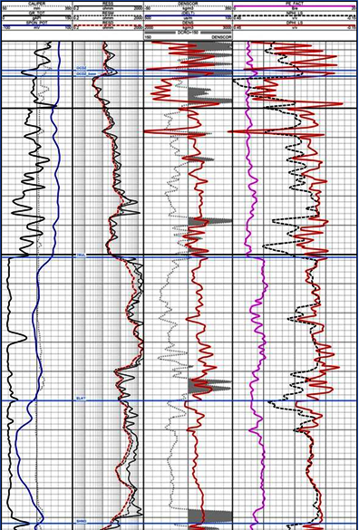
Example of log reconstruction in a shaly sand sequence (Dunvegan).
The 3 tracks on the left show the measured gamma ray, caliper,
density, and compressional sonic. Original density and sonic are
shown in black, modeled logs are in colour. Shear sonic is the model
result as none was recorded in this well. Computed elastic
properties are shown in the right hand tracks. Results from the
original unedited curves are shown in black, those after log editing
are in colour. Note that the small differences in the modeled logs
compared to the original curves propagate into larger differences in
the results, especially Poisson's Ratio (PR), Young's Modulus (ED),
and total closure stress (TCS).
 Step 17: Calculate Dynamic
Mechanical Properties
The reconstructed density and sonic logs are used to calculate:
• Poisson’s ratio
R = DTS / DTC
PR = (0.5 * R^2 - 1) / (R^2 - 1)
•
Shear modulus
N = KS5 * DENS / (DTS ^ 2)
• Young’s dynamic modulus
Y = 2 * N * (1 + PR)
•
Bulk modulus
Kb = KS5 * DENS * (1 / (DTC^2) - 4/3
* (1 / (DTS^2)))
• Mullin's brittleness index
Y1 = ((Yst - 1)
/ (8 - 1) * 100)
PR1 = ((PR - 0.40) / (0.15 - 0.40)) * 100
BI = (Y1 + PR1) / 2
The equations used to generate these
values have been used for many years with well log data as
input. The results are usually called dynamic rock properties
because the sonic log is an impulse (moderately high frequency)
measurement. Dynamic measurements can also be made in the lab
using a sparker type device. Static measurements are also made
in the lab, using pressure sleeves; the process is considered to
be a zero frequency or static measurement. Unfortunately, the
dynamic and static results do not agree with each other.
Calibrate to dynamic lab data.
Read More about Dynamic Rock
Properties
Step 18: Compare Mechanical
Properties to Other Models
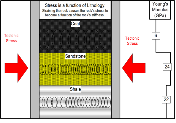
Simple linear
relationships may work well in clastic intervals, usually
relating the parameter to shale volume and mineralogy. Neural
network models may also work with corrected log data. The
results from the mechanical properties analysis should be
compared to the following graphs, based on the lithology and the
compressional sonic log values. Data that falls off trend is
probably suspect, suggesting that further log editing or
adjustments to the analysis parameters are needed.
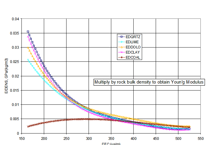
Young's Modulus versus compressional travel
time (DTS)
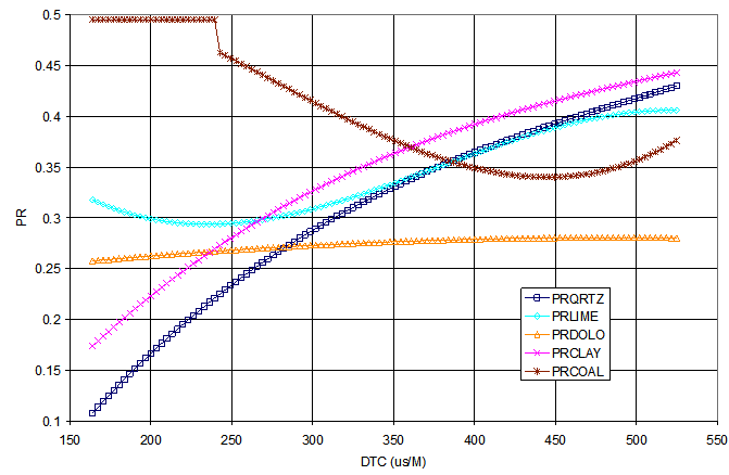
Poisson's Ratio versus compressional travel time (DTS)
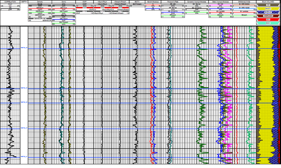
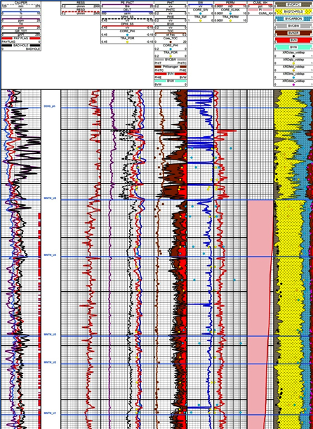
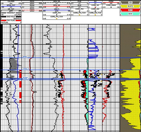
Sample of a mechanical properties log analysis. Left hand tracks show original and reconstructed logs. All results are shown in that right hand tracks. At far right is the lithology / porosity track for correlation.
 Step 19: Estimate Static Mechanical
Properties
Step 19: Estimate Static Mechanical
Properties
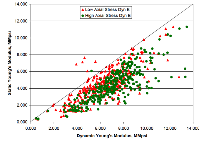
Static values differ from dynamic values because strain and strain rate are dependent on the measurement method.
• dynamic: acoustic wave propagation is a phenomenon of small strain at a large strain rate
• static (triaxial): large strain at small strain rate
Rocks appear stiffer in response
to an elastic wave, compared to a rock mechanics laboratory (triaxial)
test. The weaker the rock, the
larger the difference. This accounts for the difference
between dynamic and static Young’s moduli. The difference between dynamic
and static Poisson’s ratio is very small, and is generally not
considered.
Static mechanical rock properties are needed as input for
hydraulic fracture simulation work because static values more closely
represent the strain and strain rate created during hydraulic frac stimulation treatments.
Many transforms have been
published.
Calibrate to static lab data.
Read More about
Static Rock Properties
Step 20: Calculate
Closure Stress
Closure stress is calculated using GOHFER’S Total Stress equation and must be calibrated to local field conditions with a strain or stress correction factor. In tectonically active areas, the closure stress calculated from logs will be too low and will need to be increased. Generally, the strain offset approach is favoured.
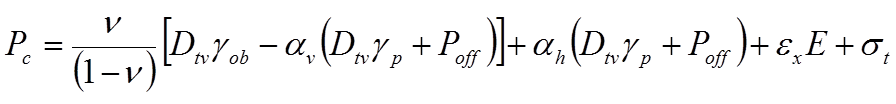
Pc = closure pressure, kPa
ν = Poisson’s Ratio
Dtv = true vertical depth, m
γob = overburden stress gradient, kPa/m
γp = pore fluid gradient, kPa/m
αv = vertical Biot’s poroelastic constant
αh = horizontal Biot’s poroelastic constant
Poff = pore pressure offset, kPa
εx = regional horizontal strain, microstrains
E = Young’s Modulus, GPa
σt = regional horizontal tectonic stress, kPa
 Overburden
Pressure:
Overburden
Pressure:
The density log is used to
calculate overburden stress. The easiest way to calculate
overburden stress is by determining the average bulk density
above treatment depth. Bad density data are first eliminated by
running a discriminator, using caliper and density correction
logs. With the discriminator
applied, the average bulk density is calculated and then used to
calculate overburden stress.
The more complicated approach
requires integration of the bulk density log. This approach requires a
synthetic density log to be created. The synthetic log is then
integrated from treatment depth to shallowest log reading.
Pore Pressure:
Field measured
data should be used to assign pore pressure. Pore fluid
supports part of the total stress. Pore pressure
depletion increases net stress and leads to compaction. Pore pressure
depletion decreases total (fracture closure) stress.
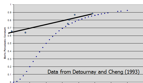 Biot’s
constant:
Biot’s
constant:
Barree defines Biot’s poro-elastic
constant as the efficiency with which internal pore pressure
offsets the externally applied vertical total stress. As Biot decreases, net (intergranular)
stress increases and pore pressure variations have less impact
on net stress.
Calibrate to mini-frac or field data.
The best way to calibrate closure
stress is to review previous fracturing work in nearby wells, or
to perform a mini-frac. If possible, this step should be
completed by the completion engineer (the person running the
hydraulic frac simulation software).
Read More about Closure Stress
STRAIN OFFSET
Calibration eXAMPLE
The following schematic examples,
prepared by Dorian Holgate, illustrate computed mechanical
properties and closure stress, and how they change with
different reservoir conditions.
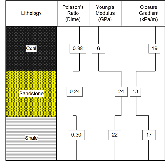
Base Case: No stress offset, no
strain offset
Regional tectonic stress added --- closure stress increases
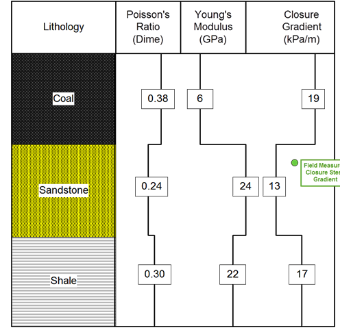

Mini-frac closure stress does not match base case
Strain offset added to calibrate to field data
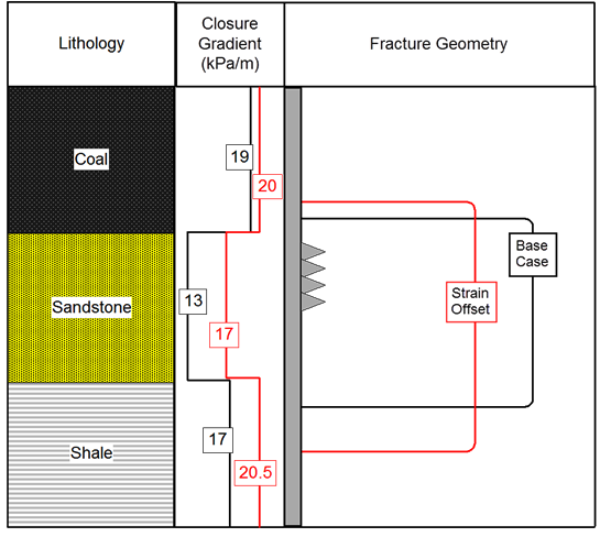
Applying a strain offset can decrease the stress difference between the reservoir and non-reservoir intervals - fracture geometry will be affected compared to base case.
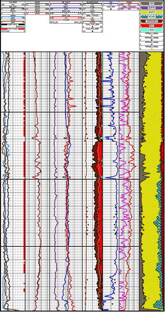
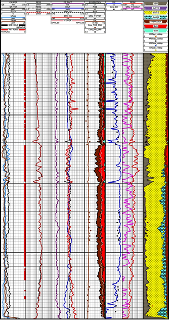
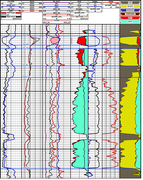
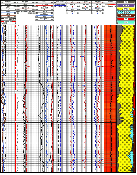
Unconventional shale gas example. Results from the custom
calculation sequence match SCAL data very well. Next, results
were used as input to reconstruct the density and sonic logs.
The reconstructed logs were then used to calculate mechanical
rock properties.
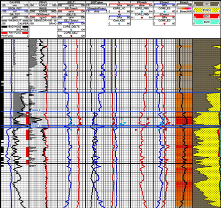
Clastic Example with Rough Bore Hole.
The reconstructed density and sonic logs were
used to calculate mechanical rock properties.
Copyright 2023 by Accessible Petrophysics Ltd.
CPH Logo, "CPH", "CPH Gold Member", "CPH Platinum Member", "Crain's Rules", "Meta/Log", "Computer-Ready-Math", "Petro/Fusion Scripts" are Trademarks of the Author