You should know the basic rules for eyeball analysis of log curves to help you climb the “Ladder to Success”. Some people find the Log Response Chart (PDF) helpful, but it requires a mental assessment of 5 or 6 log curves simultaneously. This is a little tough for novice analysts and prone to error by even the most experienced.
The step by step procedure using Crain's Rules will reduce the complexity considerably and give you a straight forward path toward your goal. The illustration below is to give you a few of the basic rules in one single illustration. Further on there is a more rves - the gamma ray (GR), resistivity, and a porosity indicating log (a sonic in this example). The GR is at the far left and the sonic is the left edge of the red shading. The resistivity and sonic have been overlaid to make it easier to see the shape of the two curves relative to each other.
Basic Rule "A": When GR (or SP) deflect to the left the zone is clean and might be a reservoir quality rock. When GR deflects to the right, the zone is usually shale (not a reservoir quality rock). There are exceptions to this rule, of course..
Basic Rule "B": Porosity logs are scaled to show higher porosity to the left and lower porosity to the right. Clean and porous is good, so compare the GR to the porosity log and mark clean+porous zones.
Basic Rule "C": Resistivity logs are scaled to show higher resistivity toward the right. Higher resistivities mean hydrocarbons or low porosity. Low resistivity means shale or water zones. So clean+porous+high resistivity are good. There are exceptions to this rule too.
The exceptions are what makes the job interesting. There are low resistivity pay zones, radioactive (high GR) pay zones, gas shales, oil shales, coal bed methane, and low porosity zones that produce for years. Some of these are shown in the illustration. See if you can figure out the logic behind each of the interpretations shown here before you move on to the more formal rules.
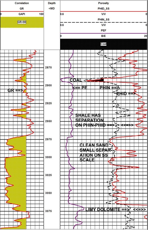
The more detailed Crain's Rules are described here with reference to the logs shown below.
Very shaly beds are not “Zones of Interest”. Everything else, including very shaly sands (Vsh < 0.50) and even obvious water zones, are interesting. Although a zone may be water bearing, it is still a useful source of log analysis information, and is still a zone of interest at this stage.
Scale the sonic log based on the assumed matrix lithology. Mark coal and salt beds, which appear to have very high apparent porosity. Identify zones which show high medium, low, or no porosity. Low porosity, high shale content, coal, and salt beds are no longer “interesting”.
OR
Low
resistivity with moderate to high porosity usually indicates
water or shale.
OR
High
resistivity with moderate to high porosity usually indicates
hydrocarbons.
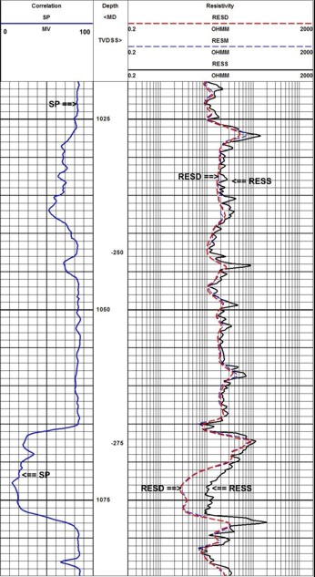
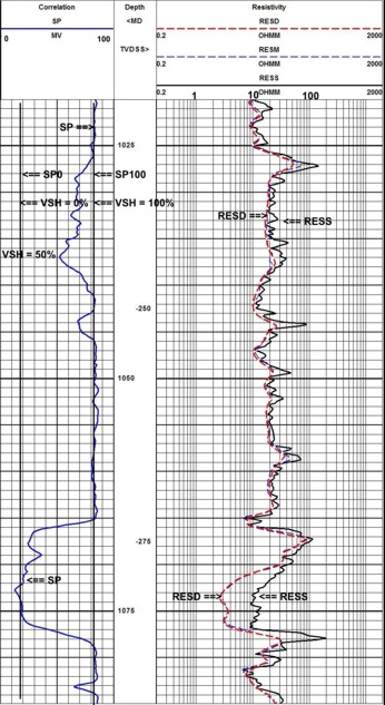
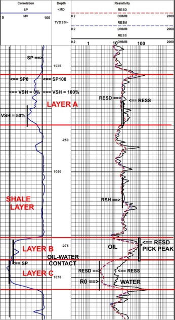
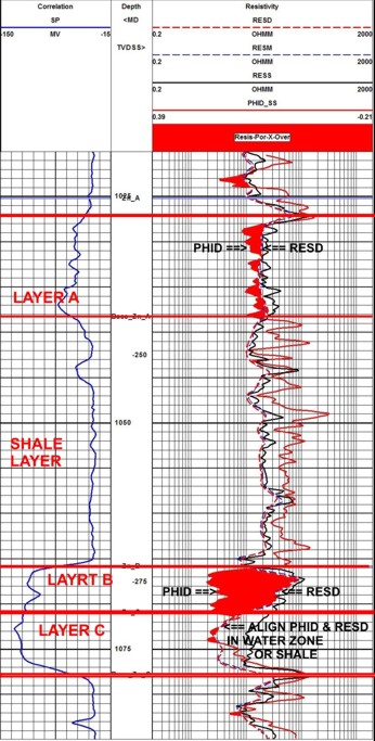
Raw logs showing resistivity porosity overlay. Red shading indicates possible hydrocarbon zones. The density or density porosity (solid red curve) is placed on top of the deep resistivity curve (dashed red curve). Line up the two curves so that they lie on top of each other in obvious water zones. If there are no obvious water zones, line them up in the shale zones. If the porosity curve falls to the LEFT of the resistivity curve, as in Layers A and B, hydrocarbons are probably present.
To find hydrocarbon indications and obvious water zones, compare deep resistivity to porosity, by mentally or physically overlaying the density porosity on top of the resistivity log. High porosity (deflections on the density log to the left) and high resistivity (deflections to the right) usually indicate oil or gas, or fresh water. See red shaded area on resistivity track on the log above.
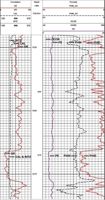
Layer A above is a shaly sand and has medium porosity. Layers B and C are clean sands and have high porosity. All other layers are shale with no useful porosity.
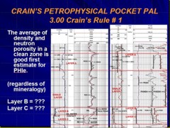
The average of density and neutron porosity in Layers B is 24 %; Layer C is 19%. This is close to the final answer because there is not much shale in these zones. The average in Layer A is 16 % - much higher than the truth due to the influence of the shale in the zone. The density porosity is about 11%, pretty close to the core data. Therefore all our analysis must make use of shale correction methods.
Low resistivity and high porosity usually means water, as in Layer C. Known DST, production, or mud log indications of oil or gas are helpful indicators.
Layer B and Layer A show crossover when the porosity is traced on the resistivity log, so these zones remain interesting. In fresher water formations, it is often difficult or impossible to spot hydrocarbons visually. If it was easy, log analysts would be out of work!
Crossover on the density neutron log sometimes means gas (not seen on the above example). Watch for rough hole problems, sandstone recorded on a limestone scale, or limestone recorded on a dolomite scale, which can also show crossover – not caused by gas.
Water zones with high porosity and low resistivity are called “obvious water zones”. Fresh water may look like hydrocarbons, particularly in shallow zones. The lack of SP development will often help distinguish fresh water zones. Low porosity water zones may not be obvious.
On Sandstone Units logs, separation for sandstone is near zero, limestone is about 7 porosity units, dolomite is 15 or more, and anhydrite is 22 or more.
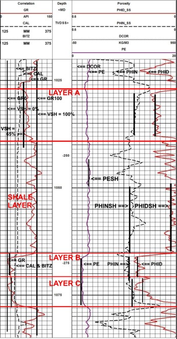
Visual determination of lithology (in addition to identifying shale as discussed earlier) is done by noting the quantity of density neutron separation and/or by noting absolute values of the photo electric curve. The rules take a little memory work.
You must know whether the density neutron log is recorded on Sandstone, Limestone, or Dolomite porosity scales, before you apply Crain’s Rule #5. The porosity scale on the log is a function of choices made at the time of logging and have nothing to do with the rocks being logged. Ideally, sand-shale sequences are logged on Sandstone scales and carbonate sequences on Limestone scales. The real world is far from ideal, so you could find any porosity scale in any rock sequence. Take care!
SANDSTONE SCALE LOG
Sand – shale identification from gamma ray and density-neutron separation. Small amounts of density neutron separation with a low gamma ray may indicate some heavy minerals in a sandstone. Most minerals are heavier than quartz, so any cementing materials, volcanic rock fragments, or mica will cause some separation. Both pure quartz (no separation) and quartz with heavy minerals (some separation) are seen.
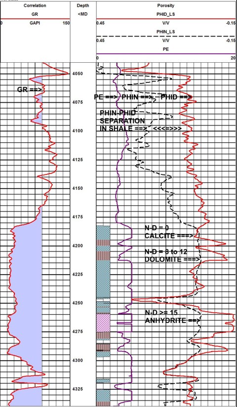
LIMESTONE SCALE LOG
The photoelectric effect is often a direct mineralogy indicator.
ROCK
N–D N–D PE GR SAND 0 - 7 2 LO LIME 7 0 5 LO DOLO 15+ 8+ 3 LO ANHY 22+ 15+ 5 LO SALT - 37 - 45 4.5 LO
SHLE 20+ 13+ 3.5 HI
THINK
LIKE A DETECTIVE:
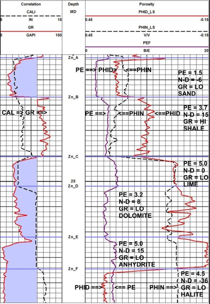
Remember: logs are not perfect and these rules are not perfect. Adjust the rules to suit your experience. Mineral mixtures are common, so think in terms of what is possible in each case.
On the
log at the right, the evidence and conclusion is shown for 6
layers with different lithology.
RULE EXCEPTIONS: High GR log readings coupled with density neutron log readings that are close together, are a sign of radioactive sandstone or limestone. To tell radioactive dolomite zones from shale zones, use a gamma ray spectral log, since the density neutron log will show separation in both cases. The PE value can help differentiate between radioactive dolomite and chlorite shale but not between dolomite and illite rich shale. High thorium values on the gamma ray spectral log indicate the shale.
To find signs of permeability, look for indications of porosity, mudcake shown by the caliper, separation on the resistivity log curves, known production or tested intervals, sample descriptions, and hydrocarbon shows in the mud.
A quicklook equation for permeability
is:
To check for indications of fractures, look for sonic log skips, density neutron crossover in carbonates, hashy dipmeter curves, hashy resistivity curves, or caved hole in carbonates.
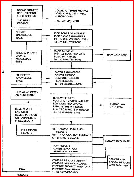
Computer systems are often provided to do the arithmetic and plot the answers. A diagram depicting the analysis steps in more detail is shown below. These steps cover only the data processing sequence involved in getting answers from the analysis of the raw data. Both novice and experienced analysts should review these illustrations to gain an understanding of how complex the processing and communication paths really are. If you use computerized log analysis, you should know how the program works.
In any step by step procedure, there is a need to calibrate each step as it is performed. This reduces labor and dead end processing paths. The control data is usually the core, test, production, geological and engineering data available from a well or its nearby offsets.
Unfortunately, much of the needed control data is not available for many zones, so calibration is seldom perfect. Even when calibration data is available, the match to log analysis results may be weak, so be prepared to use good judgment to modify or reconcile your initial assumptions to improve the comparison.
Some "ground truth", such as core data, has its
own data quality problems. It cannot and should not be used
indiscriminately to force log analysis results to some
preconceived solution. |
|
||
|
Page Views ---- Since 01 Jan 2015
Copyright 2023 by Accessible Petrophysics Ltd. CPH Logo, "CPH", "CPH Gold Member", "CPH Platinum Member", "Crain's Rules", "Meta/Log", "Computer-Ready-Math", "Petro/Fusion Scripts" are Trademarks of the Author |
|||

|
||
| Site Navigation | PETROPHYSICS COURSE CRAIN'S RULES FOR VISUAL LOG ANALYSIS | Quick Links |
 SUMMARY
OF LITHOLOGY RULES
SUMMARY
OF LITHOLOGY RULES