This page is a highly
abbreviated version of Chapter 14 on this website. For more about eater
resistivity, water saturation, alternate methods and examples, go to the
Main Index Page.
Catalogs and lab reports usually provide results at 77'F (25'C) and this value must be transformed to a different value based on the formation temperature.
STEP 1: Calculate formation temperature: 1. GRAD = (BHT – SUFT) / BHTDEP 2: FT = SUFT + GRAD * DEPTH
STEP 2: Calculate water resistivity at formation temperature: 3: RW@FT = RW@TRW * (TRW + KT1) / (FT + KT1)
Where: KT1 = 6.8 for English units KT1 = 21.5 for Metric units
If water salinity is reported instead of resistivity, as may happen in reporting direct from the well site, convert salinity to resistivity with: 4: RW@FT = (400000 / FT1 / WS) ^ 0.88
NOTE: FT1 is in Fahrenheit
In some cases, salinity is reported in parts per million Chloride instead of the more usual parts per million salt (NaCl). In this situation convert Chloride to NaCl equivalent with: 5: WS = Ccl * 1.645
To convert a downhole RW to a surface temperature, reverse the terms in equation 3: 6: RW@SUFT = RW@FT * (FT + KT1) / (SUFT + KT1)
Where: KT1 = 6.8 for English units KT1 = 21.5 for Metric units
For example, If RW@FT = 0.10 and PHIe = 0.20, then R0 = 0.10 / (0.20^2) = 2.5 ohm-m.
· Use in preference to other methods if data is available.
· Do not use if DST recovery is small; the sample may be contaminated with mud filtrate.
· Use data from last sample recovered from DST.
· Use minimum value if more than one sample or catalog value is available.
· Check chemical analysis for mud contamination.
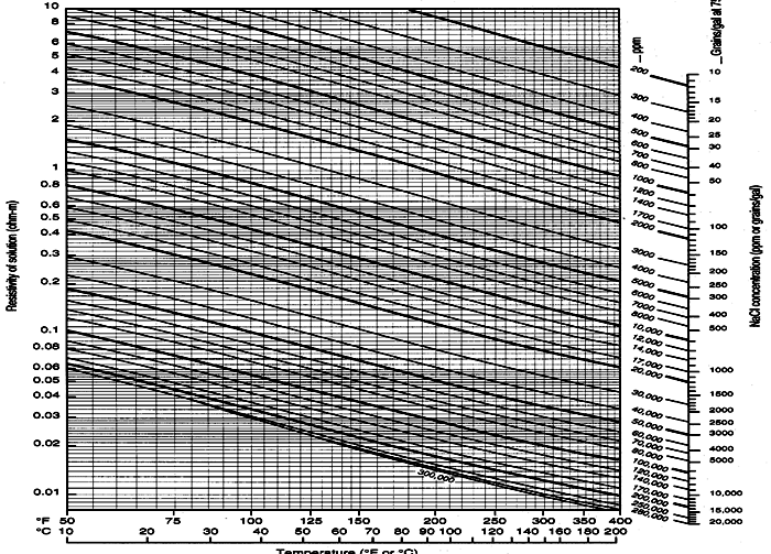
· Many people like to use the graph below to manipulate RW, temperature, and salinity.
· Compare measured lab or catalog RW values to RW from water zone method. Use your best judgment to choose one over the other.
· Plot a graph of all available temperatures versus depth (eg from log headings, DST’s, temperature logs) to obtain BT and GRAD by regression if needed. The line may not be straight. Most log heading values are too low due to cooling from mud circulation. DST values may also be low if gas expansion occurred during the test.
RW, temperature, salinity chart
If an obvious water zone exists, calculate water resistivity from the porosity and resistivity, as shown below.
STEP 1: Calculate water resistivity from an obvious water zone: 1: PHIwtr = (PHIDwtr + PHINwtr) / 2 2: RW@FT = (PHIwtr ^ M) * R0 / A
R0 is the resistivity of a known or obvious WATER layer and PHIwtr is the total porosity of the zone where R0 was chosen
If no obvious or known water zones exist, many zones may be calculated with the above equations and results scanned for low values which MIGHT be water zones. This is called the RWa method instead of the R0 method, but the math is the same: 1: RWai = (PHIti ^ M) * RESDi / A
Scan the list of Rwai values to find the minimum value of Rwa in clean, moderately high porosity zones close to the zone of interest. This Rwa value becomes RW@FT: 2: RW@FT = Min (RWai)
The above step is the equivalent to finding RW@FT directly from an "obvious" water zone: 3: RW@FT = (PHIwtr ^ M) * R0 / A
Note that this is the same as the Rwa equation, but R0, the resistivity of a defined water zone replaces RESD.
· Use in preference to SP method and to check catalog or DST values.
· Use to find RW@FT in a clean water bearing zone only. Use the result (RW@FT) to calculate water saturation in nearby hydrocarbon zones.
· Use to help calibrate A and M if RW@FT is known from DST or produced water.
· Do not attempt to find RW@FT in low porosity (less than 5%) or where shale content is high (> 20%).
· Do not attempt to find RW@FT in a hydrocarbon bearing zone.
· If zones are not "obviously" wet, calculate Rwa in many zones and scan for the minimum value. This MAY be RW@FT, but remember, there may be NO water zones in the area of your calculation, or the minimum value may be too far away to be useful.
· If there are no obvious water zones nearby, scan the well history cards or database for wells that tested water from the zone in nearby wells. Analyze logs from these wells to find RW@FT.
· To find possible hydrocarbon zones, scan for zones with Rwa greater than three times the minimum expected value.
· A shale corrected equation can be constructed by rearranging the Simandoux saturation equation.
for sandstone A = 0.62 M = 2.15 N = 2.00 for carbonates A = 1.00 M = 2.00 N = 2.00 NOTE: A, M, and N should be determined from special core analysis if possible.
If a good SP log is available, it may be used to calculate RW@FT, as shown below.
STEP 1: Calculate constants 1: GRAD1 = (BHT – SUFT) / BHTDEP 2: FT1 = SUFT + GRAD1 * DEPTH 3: KSP = 60 + 0.122 * FT1
NOTE: FT1 is in Fahrenheit
STEP 2: Calculate resistivity values 4: RSP = 10 ^ ( – SSP / KSP) 5: IF RMF@FT > 0.1 6: THEN RMFE = 0.85 * RMF@FT 7: IF RMF@FT <= 0.1 8: THEN RMFE = (1.46 * RMF@FT – 5) / (337 * RMF@FT + 77) 9: RWE = RMFE / RSP 10: IF RWE > 0.12 11: THEN RW@FT = – (0.58 - 10 ^ (0.69 * RWE – 0.24)) 12: IF RWE <= 0.12 13: THEN RW@FT = (77 * RWE + 5) / (146 – 337 * RWE)
· Do not use SP method in low porosity (less than 5%) or where shale content is high (greater than 20%).
· SP method may not work well in a hydrocarbon bearing zone.
· Do not use SP method in a carbonate or evaporite sequence.
The fifth step in a log analysis is to find water saturation. Water saturation is the ratio of water volume to pore volume. Water bound to the shale is not included, so shale corrections must be performed if shale is present. We calculate water saturation from the effective porosity and the resistivity log. Hydrocarbon saturation is 1 (one) minus the water saturation.
All methods rely on work originally done by Gus Archie in 1940-41. He found from laboratory studies that, in a shale free, water filled rock, the Formation Factor (F) was a constant defined by: 1: F = R0 / Rw
He also found that F varied with porosity: 2: F = A / (PHIt ^ M)
For a tank of water, R0 = Rw. Therefore F = 1. Since PHIt = 1, then A must also be 1.0 and M can have any value. If porosity is zero, F is infinite and both A and M can have any value. However, for real rocks, both A and M vary with grain size, sorting, and rock texture. The normal range for A is 0.5 to 1.5 and for M is 1.7 to about 3.2. Archie used A = 1 and M = 2. In fine vuggy rock, M can be as high as 7.0 with a correspondingly low value for A. In fractures, M can be as low as 1.1. Note that R0 is also spelled Ro in the literature.
For shale free rocks with both hydrocarbon and water in the pores, he also defined the term Formation Resistivity Index ( I ) as: 3: I = Rt / R0 4: Sw = ( 1 / I ) ^ (1 / N)
Archie used an N of 2 and the usual range is from 1.3 to 2.6, depending on rock texture. It is often taken to equal M, but this is not supported by core data in all cases. Rearrangement of these four equations give the more usual Archie water saturation shown in the next section.
Shale corrections are applied by adding a shale conductivity term with an associated shale porosity and shale formation factor relationship. Numerous authors have explored this approach, leading to numerous potential solutions for water saturation. Two of the most common are given in Section 8.03 and 8.04.
If you want to estimate moveable hydrocarbon, as opposed to hydrocarbons in place, you will have to calculate water saturation in the invaded zone. Water cut is derived from the differences between actual water saturation and irreducible water saturation.
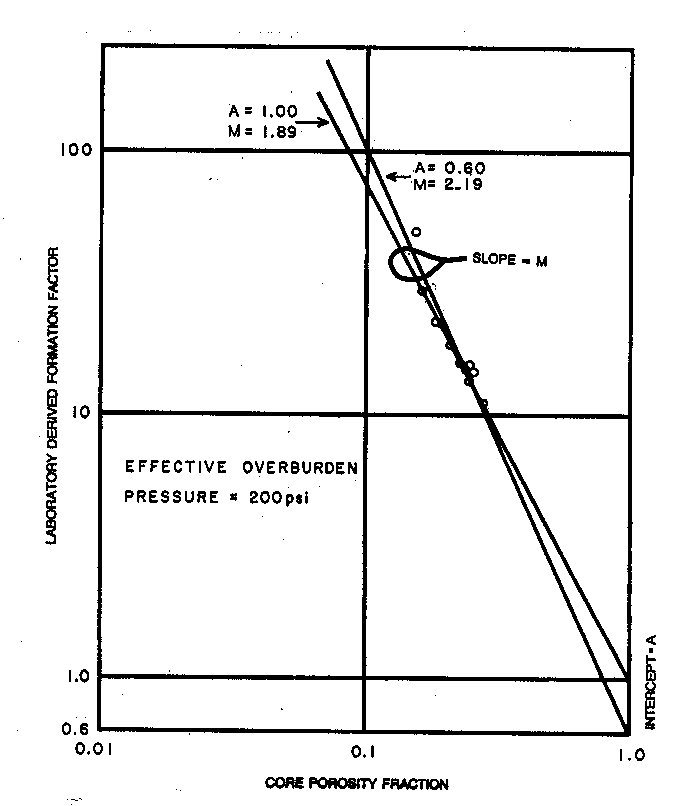
Archie initially proposed that A = 1.0, M = 2.0, and N = 2.0; later it was found that these values varied with rock type. When electrical properties are available, they should be used, provided they fall within reasonable ranges and the data set is large enough to be valid. Data is usually presented in tabular as well as graphical form, as shown below.
The slope of the best fit line through the
formation factor data is the cementation exponent, M. The best
fit line can be forced through the origin (a pinned line) which
makes the tortuosity factor A = 1.0 exactly. The intercept of
the best fit (un-pinned) line will give A; in this example A =
0.60. Data should be grouped by rock type, porosity type, or
mineralogy before the best fit lines are determined.
Formation Factor versus Porosity plot to find saturation parameters A and M
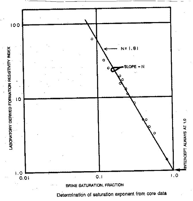
The value for the saturation exponent N is usually found in the laboratory as shown below. It is a plot of resistivity index ( I ) versus water saturation. Several partial saturations are taken on each core plug and N is determined from the slope of the line through these points. N can be varied by defining lithofacies for each core plug and relating this to some log signature. There is no equivalent crossplot to find N from log data.
The best fit line on this plot is always pinned at the origin, since resistivity index must equal 1.0 when SW = 1.0 by definition.
1: log(RESS) = – M * log(PHIe)+log(A*RMF@FT) 2: M = (log(A*RMF@FT) - log(RESS)) / log(PHIe)
A cross plot of the deep resistivity versus porosity on a log-log scale made in a clean “obvious” water zone will provide the slope M. The intercept of the line at PHIe = 1.0 is A * RW. This is called a Pickett Plot and is often a product of computerized log analysis. Shaly zones should be excluded because the shale corrected water saturation equations correct automatically for varying A and M.
Pickett plot (above) showing different slopes (M)
for
The M value in fractured rock can be quite low and compensates for the invasion of drilling fluid into the fractures. These plots are also made with shallow resistivity versus porosity. All zones are assumed to be wet due to invasion, but of course this is not true. The slope M may still be valid but the intercept is no longer A * RW, and is generally meaningless.
Pickett plot showing low values of M in fractured
The most common saturation method was developed by Gus Archie in 1941. It is widely used in all parts of the world and is suitable for carbonates, clean sands, and shaly sands where RSH is above 8 ohm-m. Where shale resistivity is low, the Archie method will be pessimistic in shaly sands.
STEP 1: Calculate water saturation: 1: PHIt = (PHID + PHIN) / 2 2: Rwa = (PHIt ^ M) * RESD / A 3: SWa = (RW@FT / Rwa) ^ (1 / N)
The term (1/N) is usually ½ or 0.5, which represents the square root. Hence: 3A: SWa = Sqrt (RW@FT / Rwa)
The water saturation from the Archie method (SWa) is called the effective water saturation, Sw.
To calculate Sxo, replace RESD with RESS and RW@FT with RMF@FT.
· The Archie method should only be used when Vsh < 0.20 and RSH > 8.0. If Vsh is high or RSH is low, then SWa is too high and a shale corrected method should be used.
· A quick look version of the Archie formula sets A = 1.0, M = 2.0 and N = 2.0.
3: SWa = (RW@FT / (PHIt ^ 2) / RESD) ^ 0.5
· This formula can be calculated by mental arithmetic or on a scratch pad when needed, and is accurate enough for quick look work.
· Calibrate water saturation to core by preparing a porosity vs SW# graph from capillary pressure data. Adjust RW, A, M, N, PHIe until a satisfactory match is achieved.
for sandstone A = 0.62 M = 2.15 N = 2.00 for carbonates A = 1.00 M = 2.00 N = 2.00 for fractured zones M = 1.2 to 1.7
NOTE: A, M, and N should be determined from special core analysis if possible.
One of the first successful shale corrected methods is this one, proposed by P. Simandoux in 1963. It reduces to the Archie formula when Vsh = 0.
STEP 1: Calculate intermediate terms: 1: C = (1 – Vsh) * A * RW@FT / (PHIe ^ M) 2: D = C * Vsh / (2 * RSH) 3: E = C / RESD
STEP 2: Calculate quadratic solution for water saturation: 4: SWs = ((D ^ 2 + E) ^ 0.5 – D) ^ (2 / N)
The water saturation from the Simandoux method (SWs) is called the effective water saturation, Sw. To calculate Sxo, replace RESD with RESS and RW@FT with RMF@FT.
· Use Simandoux method when Vsh > 0.20 and RSH < 8.0. The dual water method may also be used and the choice is usually a personal preference.
· The (2 / N) exponent in Equation 4 is an approximation and works when N is near 2. More sophisticated iterative techniques are available when N is far from 2.
· Calibrate water saturation to core by preparing a porosity vs SW# graph from capillary pressure data. Adjust RW, A, M, N, RSH, Vsh, PHIe until a satisfactory match is achieved.
RSH read from log for sandstone A = 0.62 M = 2.15 N = 2.00 for carbonates A = 1.00 M = 2.00 N = 2.00 for fractured zones M = 1.2 to 1.7
NOTE: A, M, and N should be determined from special core analysis if possible.
Another common method, based on the cation exchange capacity equation proposed by Waxman and Smits, is the Schlumberger dual water model.
STEP 1: Calculate the apparent water resistivity in shale: 0: BVWSH = (PHINSH + PHIDSH) / 2 1: RWSH = (BVWSH ^ M) * RSH / A
RWSH is a constant for each zone. Note that this is the Archie equation applied to the shale zone.
STEP 2: Calculate the resistivity of the zone as if it were 100% wet: 2: C = 1 + (BVWSH * Vsh / PHIt * (RW@FT – RWSH) / RWSH) 3: Ro = A * RW@FT / (PHIt ^ M) * C
C can be larger than 1.0 if RW@FT is greater than RWSH.
STEP 3: Calculate total and effective water saturation: 4: SWt = (Ro / RESD) ^ (1 / N) 5: SWd = (PHIt * SWt – Vsh * BVWSH) / PHIe
This equation reverts to Archie when Vsh = 0. Schlumberger uses a term called SWb, which is the bound water expressed as a saturation, and is not the same as the SWd calculated above.
The water saturation from the Dual Water method (SWd) is called the effective water saturation, Sw. To calculate Sxo, replace RESD with RESS and RW@FT with RMF@FT.
· Use Dual Water method when Vsh > 0.20 and RSH < 8.0. The Simandoux method may also be used and the choice is usually a personal preference. Dual Water may be better than Simandoux when shale resistivity is very low, eg. less than 2 ohm-m.
· The method is called the dual water method since there are two water resistivities being considered - the water in the pore space and the water bound to the shale. This is technically true of all shale corrected water saturation equations, but here the two terms are very explicitly exposed.
· The term RWSH is the apparent water resistivity (Rwa) calculated from the resistivity and the apparent porosity of the shale. It is also inverted and referred to as the conductivity of bound water (Cwb) in some technical papers.
· Exploration and development geologists often need to know how high the resistivity of a zone needs to be in order for it to be considered a potential hydrocarbon zone. The best way is to calculate the water zone resistivity (Ro) as shown above. Potential pay is indicated when RESD > 3 * Ro, water when RESD <= 2 * Ro.
· Calibrate water saturation to core by preparing a porosity vs SW# graph from capillary pressure data. Adjust RW, A, M, N, RSH, Vsh, PHIe until a satisfactory match is achieved.
RSH read from log for sandstone A = 0.62 M = 2.15 N = 2.00 for carbonates A = 1.00 M = 2.00 N = 2.00 for fractured zones M = 1.2 to 1.7 NOTE: A, M, and N should be determined from special core analysis if possible.
Most methods for calculating water saturation require the use of the resistivity log and a value for the formation water resistivity. In many cases, this latter value cannot easily be obtained from the logs directly, so for many purposes we recommend a simpler approach, namely a handy rule of thumb. The rule is based on the observation that the product of porosity and water saturation is constant for a particular zone, provided rock texture remains unchanged. The constant is called Buckles Number (KBUCKL) or the irreducible bulk volume water (BVWir).
STEP 1: Find Buckles number from special core analysis or from log analysis in a known clean pay zone that produces with zero initial water cut: 1: KBUCKL = PHIe * Sw (in a CLEAN zone which produces no initial water, or from capillary pressure data)
KBUCKL is a constant derived as above and used in the balance of the zone.
STEP 2: Solve for water saturation in each layer, but only if it is known to be a hydrocarbon zone: 2: IF Zone is hydrocarbon bearing 3: THEN SWp = KBUCKL / PHIe / (1 – Vsh) 4: OTHERWISE SWp = 1.00 5: IF SWp > 1.0 6: THEN SWp = 1.0
The water saturation from Buckles Number (SWp) is called the effective water saturation, Sw.
· Use only in pay zones at irreducible water saturation.
· If zone is water bearing, set SWp to 1.00.
· Use where RW@FT is not known.
· Do not use in heterogeneous reservoirs unless KBUCKL is also varied to match rock description.
· Buckles Number can be found by observing the porosity times water saturation product in pay zones where RW@FT is known, or where a water zone can be used to calibrate RW@FT.
· KBUCKL can also be found from capillary pressure data by averaging the product of minimum wetting phase saturation and core plug porosity for a number of samples.
· The (1 – Vsh) term can be replaced by (1 – Vsh^2) if needed.
· Calibrate water saturation to core by preparing a porosity vs SW graph from capillary pressure data. Adjust KBUCKL, Vsh, PHIe until a satisfactory match is achieved.
Sandstones Carbonates KBUCKL Very fine grain Chalky 0.120 Fine grain Cryptocrystalline 0.060 Medium grain Intercrystalline 0.040 Coarse grain Sucrosic 0.020 Conglomerate Fine vuggy 0.010 Unconsolidated Coarse vuggy 0.005 Fractured Fractured 0.001 Use these parameters only if no other source exists.
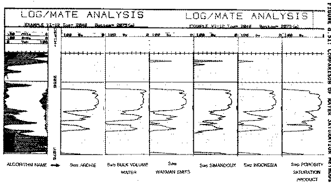
Water saturation is usually trimmed between 0.02 and 1.00. Results from a number of different methods are shown below.
Comparison of various water saturation methods
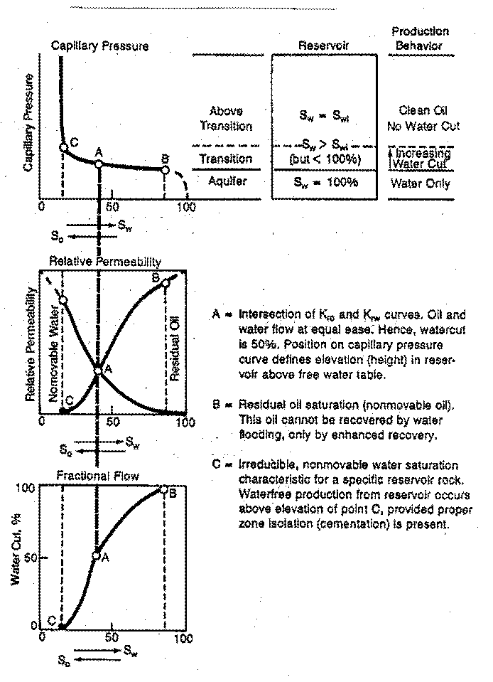
Hydrocarbon zones with water saturation (Sw) above irreducible saturation (SWir) will produce some water along with hydrocarbons. This can occur in transition zones between the oil and water leg, or after water influx into a reservoir due to production of oil or gas.
Capillary pressure curves define irreducible water saturation SWir (vertical dashed line near left edge of graph). Irreducible water saturation varies inversely with porosity: Sw = Constant / Porosity, but the Constant can vary with pore geometry. A reservoir with Sw > SWir will produce some water with the hydrocarbons.
The difference between Sw and SWir, and relative permeability of water and hydrocarbon, determine the water cut. These concepts are best described by the capillary pressure curve and relative permeability curves illustrated above.
Irreducible water saturation is a necessary value for water cut and permeability calculations.
STEP 1: Find Buckles number from special core analysis or from log analysis in a known clean pay zone that produced initially with zero water cut. 1: KBUCKL = PHIe * Sw (in a CLEAN zone that produced initially with no water, or from core data)
STEP 2: Solve for irreducible water saturation in each zone. 2: IF zone is obviously hydrocarbon bearing 3: THEN SWir = Sw 4: OTHERWISE SWir = KBUCKL / PHIe / (1 – Vsh) 5: IF SWir > Sw 6: THEN SWir = Sw
An easier,
but equivalent, model is:
· Use always in preparation for permeability calculations.
· Buckles Number can be found by observing the porosity times water saturation product in pay zones where RW@FT is known, or where a water zone can be used to calibrate RW@FT. Data can also be found from capillary pressure data.
· If Sw is greater than SWir, then the zone will produce with some water cut (if it produces anything at all).
· If Sw is less than SWir, then the Buckles number for the layer is wrong.
· The (1 – Vsh) term can be replaced by (1 – Vsh^2) if needed.
· Calibrate water saturation to core by preparing a porosity vs SWir graph from capillary pressure data. Adjust KBUCKL, Vsh, PHIe until a satisfactory match is achieved.
Sandstones Carbonates KBUCKL Very fine grain Chalky 0.120 Fine grain Cryptocrystalline 0.060 Medium grain Intercrystalline 0.030 Coarse grain Sucrosic 0.020 Conglomerate Fine vuggy 0.010 Unconsolidated Coarse vuggy 0.005 Fractured Fractured 0.001
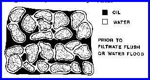
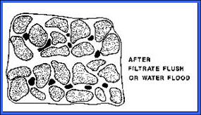
The process of drilling fluid invasion into the formation displaces oil or gas much the same as water influx from an aquifer or a waterflood. The oil or gas that is swept ahead of the invasion is called moveable hydrocarbons. That left behind is called residual oil or residual gas.
Because we record resistivity logs at different depths of investigation, we can calculate water saturation close to the borehole as well as in the undisturbed formation. The difference between the shallow and deep saturation tells us how much oil has moved. The shallow water saturation, called Sxo, is obtained from the same equation as used for Sw but RW @ FT is replaced by RMF@FT and RESD is replaced by RESS. Then: 1: Smo = Sxo – Sw 2: Sro = 1 – Sxo
· Invasion must be deeper than the zone investigated by the shallow resistivity.
· Invasion must not be too deep and affect the deep resistivity.
· These conditions are rare so Smo is not accurate in many cases.
· Verify that Sxo = Sw = 1.0 in water zones; adjust RMF and/or RW to achieve a reasonable result.
·
Set RMF = 10 to kill Smo and Sro calculations in
computer programs that insist on presenting this answer even
when the answer is wrong. |
|
||
|
Page Views ---- Since 01 Jan 2015
Copyright 2023 by Accessible Petrophysics Ltd. CPH Logo, "CPH", "CPH Gold Member", "CPH Platinum Member", "Crain's Rules", "Meta/Log", "Computer-Ready-Math", "Petro/Fusion Scripts" are Trademarks of the Author |
|||

|
||
| Site Navigation | PETROPHYSICS COURSE HOW TO CALCULATE WATER SATURATION | Quick Links |

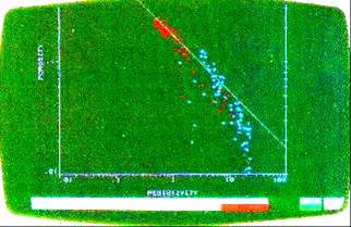 The
Pickett plot can be used to find A and M from log data, instead
of core data. In hydrocarbon zones, we assume the flushed zone
is nearly 100% wet, and re-arrange the Archie equations as
follows:
The
Pickett plot can be used to find A and M from log data, instead
of core data. In hydrocarbon zones, we assume the flushed zone
is nearly 100% wet, and re-arrange the Archie equations as
follows: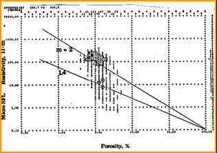 dolomite
(red) and limestone (blue) in a single reservoir
dolomite
(red) and limestone (blue) in a single reservoir PARAMETERS: