QUICKLOOK WELL LOG OVERLAYS

Most people working in the oil industry just want to "look" at a log and understand what the reservoir is all about. Even after years of experience, this is difficult, especially when working on new or unfamiliar areas. That's why specialists use fancy software and take hours or days to generate results for the rest of the team.

However, there are things you can do using your eyes and your logical brain power to gain some understanding without the calculator or the chartbook.

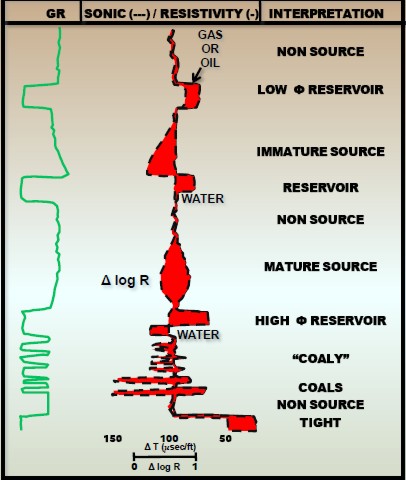
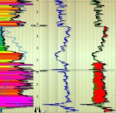
Lets start with just 3 curves - the gamma ray (GR), resistivity, and a porosity indicating log (a sonic log in this case) as shown in the image below. The GR is at the far left and the sonic is the left edge of the red shading. The resistivity and sonic have been overlaid to make it easier to see the shape of the two curves relative to each other.

Basic Rule "A": When GR (or SP) deflect to the left the zone is clean and might be a reservoir quality rock. When GR deflects to the right, the zone is usually shale (not a reservoir quality rock). There are exceptions to this rule, of course.

Basic Rule "B": Porosity logs are scaled to show higher porosity to the left and lower porosity to the right. Clean and porous is good, so compare the GR to the porosity log and mark clean+porous zones.

Basic Rule "C": Resistivity logs are scaled to show higher resistivity toward the right. Higher resistivities mean hydrocarbons or low porosity. Low resistivity means shale or water zones. So clean+porous+high resistivity are good. There are exceptions to this rule too.

Schematic drawing of a resistivity-porosity overlay, showing the variety of rocks that can show separation between the porosity and resistivity. Note that the two curves "track" each other in water and non-source shales.

The exceptions are what makes the job interesting. There are low resistivity pay zones, radioactive (high GR) pay zones, gas shales, oil shales, coal bed methane, and low porosity zones that produce for years. Some of these are shown in the illustration. See if you can figure out the logic behind each of the interpretations shown here before you move on to the more formal rules.

The technique is called the resistivity-porosity overlay. It has been in use since about 1962 when the first sonic logs showed up, concurrent with the beginning of the logarithmic scale for resistivity log displays.

The overlay is created by tracing or "overlaying" the deep resistivity curve (on a logarithmic scale) on top of a porosity log (sonic, density, or neutron), and shifting the resistivity log sideways until it lines up with the porosity curve in an "obvious" water zone. That means that the lowest resistivity values sit on top of the porosity curve and higher resistivity values fall to the right of the porosity curve. We then colour in the separation between the curves with a red pencil, and perforate the zone for production.

If there is no obvious water zone, we do the overlay using a nearby (non-source rock) shale bed instead - less accurate but it works often enough. The concept is widely used to identify source rocks. Some of these are completed as unconventional reservoirs such as the Barnett Shale (resistive shales).

SOME OVERLAY EXAMPLES

Most overlays also show the SP and GR logs to aid in correlation and to recognize cleaner rocks form shalier rocks. Here are some examples.

Sonic resistivity overlay showing separation in Barnett Shale, Texas, labeled "ΔlogR" and shaded red. The high resistivity interval is about 50% clay and 50% silt with 4 to 5% porosity, with free gas and adsorbed gas. There is kerogen, as well as gas, contributing to the high resistivity. The zone is also quite radioactive , some of it due to clay but most of it due to uranium carried by the kerogen.

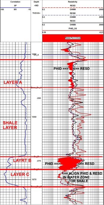
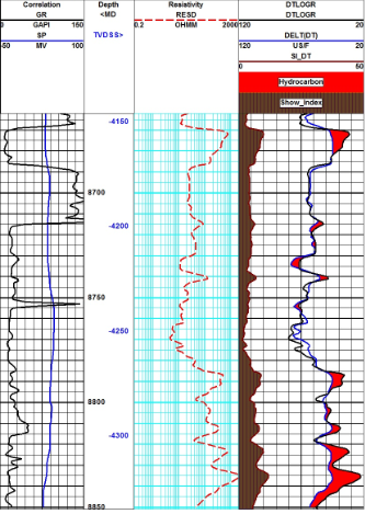
Raw logs showing resistivity porosity overlay. Red shading indicates possible hydrocarbon zones. The density or density porosity (solid red curve) is placed on top of the deep resistivity curve (dashed red curve) Line up the two curves so that they lie on top of each other in obvious water zones. If there are no obvious water zones, line them up in the shale zones. If the porosity curve falls to the LEFT of the resistivity curve, as in Layers A and B, hydrocarbons are probably present.

Because of poorly chosen shift criteria, it is possible to create too much or too little separation between the resistivity and porosity curves. This is where the logic comes into play. If the two cureves are "tracking" each other, then the zone is wet. Tracking means the two curves roughly parallel each other, like railroad tracks. If the two curves are roughly a mirror image of each other, then they are not tracking, and separation is expected. Adjust the shift to make this happen. The quantity of the separation is a measure of the quality of the hydrocarbon show.

QUANTIFYING THE OVERLAY CONCEPT

The resistivity porosity overlay was, and still can be, made by tracing one curve on the other, or by using a film copy of one curve laid on the paper copy of the other. Back in the day, we used light tables or windows so we could see through the paper. When I traveled to the Arctic, I built a page sized light table in my brief case. The remaining space held pencils, straight edge, calculator, QC and analysis forms, spare socks, and underwear. 

Today, we can make these overlays on most professional petrophysical software packages or even with a spreadsheet program.

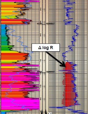
Original sonic log (black curve) and calculated resistivity curve (shaded red) showing potential source rock or, as in this case, a gas shale (Barnett)

Example of a resistivity porosity overlay looking for bypassed pay in a limestone. The resistivity has been transformed into a sonic log by appropriate scaling (see below). Red shading indicates possible hydrocarbons. The brown shaded curve is a "Show Index" - higher values are good news..

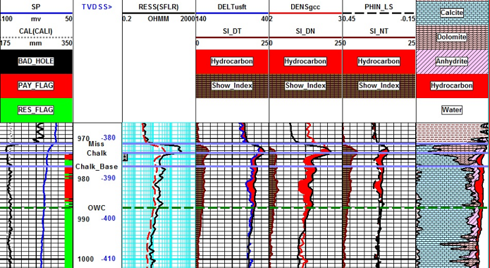
Resistivity porosity overlay for sonic, density, and neutron (shaded red) and Show Index for each (shaded brown) The full blown lithology porosity track on the right shows a typical computerized analysis. More detailed porosity, water saturation, and permeability curves would normally be presented. Here, the objective is to locate the oil water contact in a low permeability regime with residual oil below the contact. The transformed resistivity sits on the porosity curve at the base of each track (water zone) and also in the shale zone above the oil (on sonic and neutron only).

QUANTIFYING THE OVERLAY

The illustrations in the previous Section were generated by appropriate mathematical transforms that convert the resistivity log into sonic, density, and neutron values. This is easily done on most petrophysical software by adjusting the horizontal scale of the resistivity log and placing the curve in the porosity track or vice versa. A more useful approach is to code a few custom equations into the User Defined Equation module of your software. This allows you to run several dozen wells in a day to see which ones might have bypassed pay. The equations you need are:
      1: DTlogR = DT1 -- DT2 * log(RESD)
      2: SI_DT = 5 * (log(RESD / RSH) + 0.02 * (DTC -- DTCSH)

      3: DNlogR= DN1 -- DN2 * log(RESD)
      4: SI_DN = 5 * (log(RESD / RSH) - 2.5 * (DENS -- DENSSH))

      5: NTlogR = NT1 -- NT2 * log(RESD)
      6: SI_NT = 5 * (log(RESD / RSH) + 4.0 * (PHIN -- PHINSH))

Where:
  XXlogR = resistivity log scaled into compatible porosity log units
  SI_XX = show index based on the separation between the porosity log curve and the transformed resistivity

Default Values for Carbonates:

   RSH = 4.0, DTCSH = 60, DENSSH = 2.47, PHINSH = 0.15
   DT1 = 82, DT2 = 22, DN1 = 2.10, DN2 = --0.45, NT1 = 0.22, NT2 = 0.09
 

The parameters assume DTC is in usec/ft, DENS is in g/cc, and PHIN is decimal fraction porosity.

Shale base lines need to be adjusted so that the Show Index is near zero in water or shale zones.

DT1, DN1, NT1 are adjusted so that the resistivity porosity separation is near zero in shale or water zones.
DT2, DN2, NT2 are amplitude scale factors and seldom need to be changed.

Default shale base lines for sand shale sequences will be considerably higher.

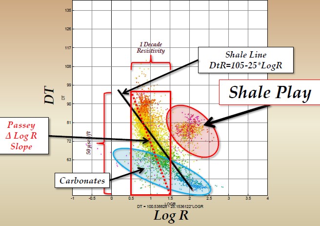
The best way to find the parameters for scaling resistivity into porosity units is to crossplot logarithm of resistivity on the horizontal axis and the porosity indicating log values on the vertical axis. You need to include enough interval to see non-source rick "normal" shales and some of the potential reservoir intervals. The data points along the southwest edge of the data show the normal trendline. Data points for reservoir or source rock peel off toward the northeast of the plot area.

Sonic versus logarithm of resistivity (DTlogR) Crossplot showing non-source rock trend line and reservoir or source rock clusters of data. The equation of the non-source rock line is DTlogR = 105 - 25 log(RESD) for this Barnett Shale example (DT1 = 105 and DT2 = 25). Similar plots can be made with density or neutron data on the vertical axis..