The physical model shown
below is critical in the understanding of how logs respond to the
different components of the rock. To see the effect of variations in
lithology, porosity, and fluid type, see
Log Response Chart (PDF).
You will need to view this file at 100% zoom in Acrobat to read the
curves. Remember that the density and neutron are shown on a
Limestone equivalent scale, so sandstones show crossover even when
there is no gas.
This response equation will work for sonic travel time, density, or density porosity, neutron porosity, gamma ray (and the spectrolog curves - uranium, thorium and potassium), resistivity (if Sxo is replaced by Sw for deep resistivity logs), the electromagnetic propagation log, the thermal decay time log, and the photoelectric effect (if PE * DENS is used). It will also work for various derived logs described in later chapters of this handbook. The response equations can be used in several ways. One is to find out what a log would read under a hypothetical set of circumstances. Another way is to calculate one unknown in the equation, for example porosity or shale volume, by using a log reading and assuming the other terms to be known or derivable from some other response equations. A third approach is to use sets of response equations simultaneously to determine as many unknowns as possible from the available log data. Some terms in the response equation for certain logs go to zero. This is what makes it possible, for example, to calculate the shale volume from the gamma ray response. Both the water and hydrocarbon terms go to zero, since neither of these components has any gamma ray contribution. By re-arranging terms and further assuming that porosity is small, we get: 1. VSHgr = (GR - GRmatrix) / (GRshale - GRmatrix) Here GR, GRshale, and GRmatrix are read from appropriate places on the gamma ray log to calculate shale volume. In other cases, we sometimes lump two terms together, as for water and oil in the sonic log equation for porosity. This strategy eliminates the need to know water saturation prior to knowing porosity. This approach will fail if gas is present because the water and gas contributions are too dissimilar. The algorithms in following chapters attempt to resolve as many of the unknowns as possible using these piecewise techniques. Where this is inappropriate, sets of two or three simultaneous equations are solved, with the final solution being given. It will not always be obvious that simultaneous response equations were used, but ALL deterministic log analysis methods rely on this approach. What we have done here is eliminate the repetitive derivation of the solution, and present instead the finished product, ready for inclusion in a calculator, spreadsheet or computer program.
The
borehole environment, invasion, and rock model define the log
analysis problem. Logging tools define most of the data available
to analyze the model. With many analysis methods to choose from,
there are usually many possible answers. It is the analyst's job
to select the method and model that best describe the problem
to be solved. Adjustments to the basic model presented here are
therefore plausible, and may be essential. |
|
||||||||||||||||
|
Page Views ---- Since 01 Jan 2015
Copyright 2023 by Accessible Petrophysics Ltd. CPH Logo, "CPH", "CPH Gold Member", "CPH Platinum Member", "Crain's Rules", "Meta/Log", "Computer-Ready-Math", "Petro/Fusion Scripts" are Trademarks of the Author |
|||||||||||||||||

|
||
| Site Navigation | PETROPHYSICS COURSE THE LOG RESPONSE EQUATION | Quick Links |