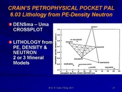
We can solve for the volume of one mineral for each porosity indicating log over the zone. Thus a sonic, density, neutron combination or photoelectric effect, density, neutron combination can provide volumes for either two or three mineral models. YOU must choose the correct two or three minerals for the end points of the model. Choosing the wrong end points may lead to mathematically feasible results which are not correct.
If additional lithology indicating curves are available, for example the natural or induced spectral gamma ray logs, one more mineral may be added to the model for each useable curve. Such models cannot be computed by hand, and computer programs are required. {n some software, porosity can be one of the “minerals”.
When gas is present, only the photo electric effect (two mineral model) is useful for hand calculated lithology analysis. If only one porosity indicating log is present, the lithology will be, by definition, the lithology you imposed on the porosity calculation done earlier.
The META/ESP spreadsheet, available on the Downloads tab at www.spec2000.net, handles these models and makes the work relatively painless.
This is the easiest and most common lithology method and is widely used in wellsite and office computer programs.
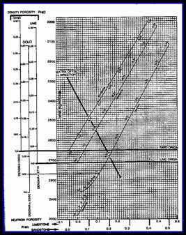
STEP 1: Calculate shale density from shale porosity (a constant for each zone): 1: DENSSH = PHIDSH * KD1 + (1 – PHIDSH) * KD2
PHIDSH and DENSSH are constants for each zone, chosen from the density log in a nearby shale.
STEP 2: Translate density porosity for each layer to density units: 2: DENS = PHID * KD1 + (1 – PHID) * KD2
KD1 = 1000 for Metric units KD2 = 2.65 for English units Sandstone scale log KD2 = 2650 for Metric units Sandstone scale log KD2 = 2.71 for English units Limestone scale log KD2 = 2710 for Metric units Limestone scale log KD2 = 2.87 for English units Dolomite scale log KD2 = 2870 for Metric units Dolomite scale log
STEP 3: Calculate matrix density:
3: DENSma =
(DENS – PHIe * DENSW – Vsh * DENSSH)
STEP 4: Calculate rock volumes: 4: Min1 = (DENSma – DENS2) / (DENS1 – DENS2) 5: Min2 = 1.0 – Min1
To use this method for sonic neutron crossplot, replace all DENSxx terms in Equations 3, 4, and 5 with their corresponding DTCxx terms. Equations 1 and 2 are not needed.
· If Min1 and Min2 are to be plotted in a volumetric track with Vsh and PHIe, multiply by Vrock before plotting, where Vrock = 1 – PHIe – Vsh.
· Use any time data is available, but not in bad hole conditions or when gas is present. Methods using PE or UMA are usually better.
· This equation will break down when PHIe plus Vsh approaches 1.0, so we limit the use of the equation to those cases where PHIe + Vsh < 0.8.
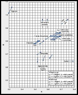
This is usually called the M-N method in the literature. This method provides two different two-mineral and one three-mineral models.
YOU must choose the model which gives the best resolution for the mineral end points you have chosen. Resolution is better when the values for the end points have the largest absolute difference.
STEP 1: Shale correct log data: 1: PHIdc = PHID – (Vsh * PHIDSH) 2: PHInc = PHIN – (Vsh * PHINSH)
If PHIN is in sandstone units, subtract 0.03 before using it. 3: PHIsc = (DTC – (1 – Vsh) * 47.3 – (Vsh * DTCSH)) / (KS1 – 47.3)
Note: DTC must be in English units (us/ft). 4: DENSc = PHIdc * KD1 + (1 – PHIdc) * 2.71 5: DTCc = PHIsc * KS1 + (1 – PHIsc) * 47.3
KD1 = 1.1 for salty drilling mud KS1 = 200 for fresh drilling mud KS1 = 188 for salty drilling mud
STEP 2: Calculate lithology factors: 6: Mlith = 0.01 * (KS1 – DTCc) / (DENSc – KD1) 7: Nlith = (1.00 - PHInc) / (DENSc – KD1) 8: Klith = Mlith / Nlith 9: Alith = 1 / Nlith
STEP 3: Calculate two mineral rock volumes from MLITH factor: 10: Min1 = (Mlith – MLITH2) / (MLITH1 – MLITH2) 11: Min2 = 1.0 – Min1
STEP 4: Calculate two mineral rock volumes from NLITH factor: 12: Min1 = (Nlith – NLITH2) / (NLITH1 – NLITH2) 13: Min2 = 1.0 – Min1
STEP 5: Calculate three mineral rock volumes from Mlith and Nlith: 14: D = (Mlith * (NLITH2 – NLITH1) + Nlith * (MLITH1 – MLITH2) + MLITH2 * NLITH1 – MLITH1 * NLITH2) / (MLITH1 * (NLITH3 – NLITH2) + MLITH2 * (NLITH1 – NLITH3) + MLITH3 * (NLITH2 – NLITH1))
15: E = (D * (NLITH3 – NLITH1) – Nlith + NLITH1) / (NLITH1 – NLITH2) 16: Min1 = MAX(0, 1 – D – E) / (MAX(0, 1 – D – E) + MAX(0, D) + MAX(0, E)) 17: Min2 = MAX(0, E) / (MAX(0, 1 – D – E) + MAX(0, D) + MAX(0, E)) 18: Min3 = 1 – Min1 – Min2
SPECIAL CASES:
Cannot be used in gas zones.
To use DTCma and DENSma instead of Mlith and Nlith, replace all Mlith terms with DTCma terms, and all Mlith with DENSma terms in Equations 15 and 16. Equations 1 thru 14 are not needed, but DTCma and DENSma must be derived as shown in Section 6.01.
· If Min1 and Min2 are to be plotted in a volumetric track with Vsh and PHIe, multiply by Vrock before plotting, where Vrock = 1 - PHIe – Vsh. For examp;e Vmin1 = Min1 * Vrock.
· Nlith gives about the same answer as the matrix density method, because both methods use density and neutron data. Do not use in bad hole conditions or when gas is present.
· Mlith uses sonic and density data. Do not use in bad hole conditions or when gas is present.
· Alith and Klith can be used to calculate 2 or 3 mineral models by replacing all Mlith and Nlith terms in Equations 10 through 18 with corresponding Alith and Klith terms.
· Klith uses sonic and neutron data and can be used in bad hole where Mlith and Nlith are no good.
· For the available two or three mineral models in this section, choose the method with the most resolution for the mineral pair you have chosen. This means that the numerical distance between the end points is as large as possible.
· Mlith and Nlith are usually called M and N, but they can be confused with the cementation exponent M and the saturation exponent N, so we have changed their names to reduce confusion.
To calculate MLITH and NLITH parameters for salt mud case, use Equations 6 and 7 with KD1 and KS1 for salt mud.
This is the best method for calculating lithology if the data is available. This method provides two different two-mineral and one three-mineral models.
YOU must choose the model which gives the best resolution for the mineral end points you have chosen. Resolution is better when the values for the end points have the largest absolute difference.
STEP 1: Calculate shale density and shale capture cross section (a constant for each zone): 1: DENSSH = PHIDSH * KD1 + (1 – PHIDSH) * KD2 2: USH = PESH * DENSSH
STEP 2: Translate density porosity to density units for each layer: 3: DENS = PHID * KD1 + (1 – PHID) * KD2
Where: KD1 = 1.00 KD2 = 2.65 for Sandstone scale KD2 = 2.71 for Limestone scale
NOTE: Density data is needed in English units (gm/cc).
STEP 3: Calculate matrix capture cross section for each layer: 4: Uma = (PE * DENS – Vsh * USH) / (1 – PHIe)
STEP 4: Calculate two mineral rock volumes from UMA: 5: Min1 = (Uma – UMA2) / (UMA1 – UMA2) 6: Min2 = 1.0 – Min1
STEP 5: Calculate two mineral rock volumes from PE: 7: Min1 = (PE – PE2 – PESH * Vsh) / (PE1 – PE2) 8: Min2 = 1.0 – Min1
STEP 6: Calculate three mineral rock volumes from Uma and DENSma: 9: D = (Uma * (DENS2 – DENS1) + DENSma * (UMA1 – UMA2) + UMA2 * DENS1 – UMA1 * DENS2) / (UMA1 * (DENS3 – DENS2) + UMA2 * (DENS1 – DENS3) + UMA3 * (DENS2 –DENS1))
10: E = (D * (DENS3 – DENS1) – DENSma + DENS1) / (DENS1 – DENS2) 11: Min1 = MAX(0, 1 – D – E) / (MAX(0, 1 – D – E) + MAX(0, D) + MAX(0, E)) 12: Min2 = MAX(0, E) / (MAX(0, 1 - D - E) + MAX(0, D) + MAX(0, E)) 13: Min3 = 1 – Min1 – Min2
Only the PE 2 mineral model can be used in gas zones.
To use DTCma instead of Uma, replace all Uma terms with DTCma terms in Equations 9 and 10. Equations 1 thru 8 are not needed, but DTCma and DENSma must be derived as shown in Section 6.01.
· If Min1 and Min2 are to be plotted in a volumetric track with Vsh and PHIe, multiply by Vrock before plotting, where Vrock = 1 - PHIe – Vsh.For example, Vmin1 = Min1 * Vrock.
· Use the Uma method any time data is available, but not in bad hole conditions or when gas is present.
· Use the PE method any time data is available, but not in bad hole conditions. However it can be used when gas is present.
· There may be three mineral combinations where the sonic density neutron methods have better resolution. Check the shape of the mineral triangles.
· Porosity can also be obtained from the PE response equation. Since resolution is poor, this method is not recommended – the density/PE combination is better.
· If this method is used to find the fraction of clay minerals present in a shale, Uma is found from Uma = PESH * DENSsh / (1 - BVWSH). Then the two or three mineral model is applied.
· If natural gamma ray spectral log data is available, other two and three mineral models can be solved in similar fashion as for PE density neutron.
· If clay is to be one of the minerals to be found along with two matrix rocks, then do not shale correct the Uma equation, and use PHIt instead of PHIe in Step 2.
* PHINMA DENSMA DTCMA MLITH NLITH PE UMA Clean Quartz – 0.028 2650 182 0.802 0.623 1.82 4.8 Calcite 0.000 2710 155 0.822 0.585 5.09 13.8 Dolomite 0.005 2870 144 0.769 0.532 3.13 9.0 Anhydrite 0.002 2950 164 0.707 0.512 5.08 15.0 Gypsum 0.507 2350 172 1.002 0.365 4.04 9.5 Mica Muscovite 0.165 2830 155 0.768 0.456 2.40 6.8 Biotite 0.225 3200 182 0.601 0.352 8.59 27.5 Clay Kaolinite 0.491 2640 211 0.753 0.310 1.47 3.9 Glauconite 0.175 2830 182 0.723 0.451 4.77 13.5 Illite 0.158 2770 212 0.696 0.476 3.03 8.4 Chlorite 0.428 2870 212 0.658 0.306 4.77 13.7 Montmorillonite 0.115 2620 212 0.760 0.546 1.64 4.3 Barite 0.002 4080 229 0.383 0.324 261 1065 NaFeld Albite – 0.013 2580 155 0.889 0.641 1.70 4.4 Anorthite – 0.018 2740 148 0.820 0.585 3.14 8.6 K-Feld Orthoclase – 0.011 2540 226 0.772 0.656 2.87 7.3 Iron Siderite 0.129 3910 144 0.494 0.299 14.3 56.2 Ankerite 0.057 3080 150 0.683 0.453 8.37 25.8 Pyrite – 0.019 5000 130 0.370 0.255 16.4 82.2 Evaps Fluorite – 0.006 3120 150 0.670 0.475 6.66 20.8 Halite – 0.018 2030 220 1.172 0.988 4.72 9.6 Sylvite – 0.041 1860 242 0.295 0.270 8.76 16.3 Carnalite 0.584 1560 256 1.959 0.743 4.29 6.7 Coal Anthracite 0.414 1470 345 1.757 1.247 0.20 0.3 Lignite 0.542 1190 525 1.460 2.411 0.25 0.3
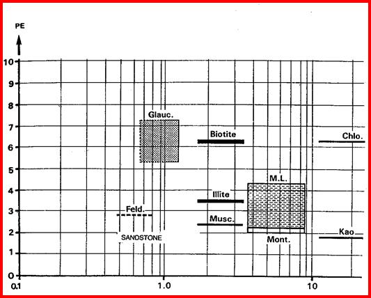
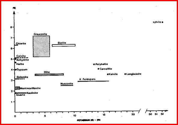
Many other two and three mineral models can be made using combinations of sonic, density, neutron, PE and spectral gamma ray log curves, such as potassium or thorium or potassium/thorium ratio. Typical crossplots are shown on the following page.
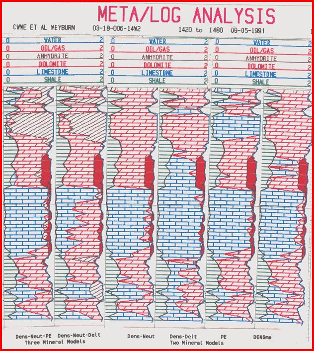
A comparison of various lithology methods is shown on Figure PP6.19. Notice that some models could not resolve for three minerals so the anhydrite zone is not portrayed correctly.
PE vs Th/K Ratio Crossplot for Lithology. X Axis Th/K (ppm/%)
PE vs Potassium Crossplot for Lithology. X Axis is K (%).
Comparison of Lithology Methods. Note that the 2-mineral model will give silly results in a 3-mineral environment, as shown here in the anhydrite layer, unless appropriate parameters and zoning are applied.
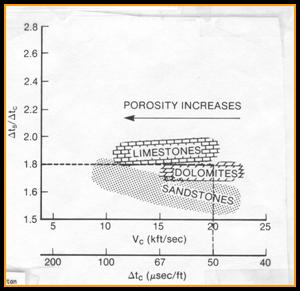
1: Vp/Vs = DTS / DTC
Where DTC = compressional travel time (usec/ft or usec/m) DTS = shear travel time (usec/ft or usec/m) Vp/Vs = velocity ratio (unitless)
This ratio is used in seismic calibration and interpretation as a guide to lithology. Vp/Vs is relatively independent of porosity and fluid type (little gas effect).
RECOMMENDED PARAMETERS: Sandstone Vp/Vs = 1.50 – 1.70 Dolostone Vp/Vs = 1.65 – 1.80 Limestone Vp/Vs = 1.80 – 2.00
|
|
|||||
|
Page Views ---- Since 01 Jan 2015
Copyright 2023 by Accessible Petrophysics Ltd. CPH Logo, "CPH", "CPH Gold Member", "CPH Platinum Member", "Crain's Rules", "Meta/Log", "Computer-Ready-Math", "Petro/Fusion Scripts" are Trademarks of the Author |
||||||

|
||
| Site Navigation | PETROPHYSICS COURSE HOW TO CALCULATE LITHOLOGY | Quick Links |
 Where:
 Where:
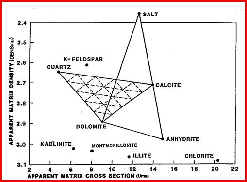
 The
dipole shear sonic log provides compressional and shear travel
time values that can be used for lithology estimation.
The
dipole shear sonic log provides compressional and shear travel
time values that can be used for lithology estimation.